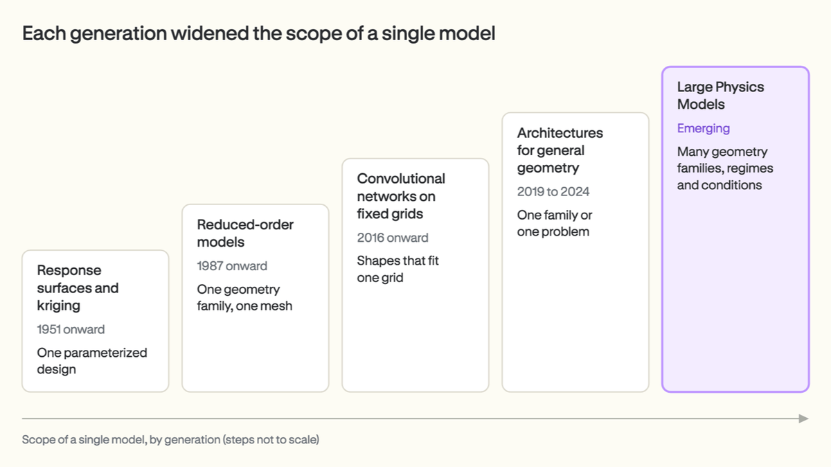
The Luminary platform’s Fall 2026 release has landed! The headline is a new agent-led experience and the introduction of Continual Large Physics Models (CLPM): with the agent-led experience, you describe the task how you would to an engineer in plain English, and Luminary’s agents carry out the work across the platform, from preparing simulation data to training models and analyzing results. CLPMs represent a step change in Physics AI, moving from static Large Physics Models, whose capabilities remain fixed once trained, to Continual Large Physics Models, whose capabilities continue to improve throughout the model’s lifetime.
If you have built a Large Physics model, you know how many steps that takes, including setting up the simulation template, meshing, launching the sweep, gathering the results, cleaning them, building the training set, training, checking the loss, running inferences, and post-processing. Because each step is manual, each handoff creates a chance for mistakes. The work also does not end once the model ships: when requirements change or a new design falls outside the training data, a static model has to go through the same manual cycle again before the model is useful.
With this release, agents take on both problems. With agentic engineering, a single plain-English request is enough for agents to plan the work across geometry, simulation, training and analysis, run it end to end, and keep working while you are away. With Continual Large Physics Models, the same agents keep the model improving after it ships by flagging where its predictions are uncertain, running the simulations that close those gaps, and updating the model with the new results without losing what it already learned, all while your team keeps using it. In both cases, the agents stop at checkpoints you define, such as a budget threshold or an ambiguity that needs your input. The handoffs that caused errors go away, and models get better instead of going stale.
Underneath the agents and the continual loop, the platform got better at every layer: more ways to generate and manage simulation data, new model architectures that are measurably more accurate, error bars and applicability checks on every prediction, and the same platform in every deployment environment.
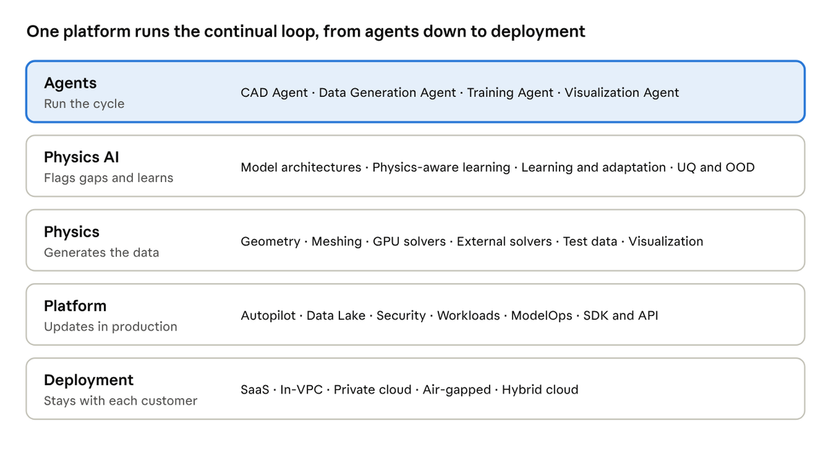
The Luminary platform stack
The sections below walk through each of these additions, starting with Continual Large Physics Models and the agent-led experience and then moving through data, models, trust, analysis and deployment. Customers can find the complete list of changes in the release notes.
New features at a glance
Continual Large Physics Models
- Continual LPMs: models that find their own coverage gaps, generate the data needed to close them, and learn that data without forgetting, all while they stay in service.
- Versioned, live updates: every loop saves a new version that is tested on the same held-out cases, and inference keeps running while the new version is promoted.
Agent-led engineering
- From one request to a finished workflow: you describe the task in plain English, and Autopilot and its subagents carry out the geometry, simulation, training and inference steps.
- Expert agents across the workflow: CAD, Data Generation, Training and Visualization agents that automate everything you need to build a Large Physics Model.
- Saved workflows: skills, notebooks and memory to capture your team’s standards and preferences so that the agents follow them consistently.
- Approval checkpoints: agents that are transparent, auditable, and permissioned, and that work within the time and compute budgets you set.
- Agents where you work: access from the web UI, the Python SDK, notebooks, MCP clients, Slack and Teams, and an Agents API for other systems.
- Model of your choice: frontier models from Anthropic, OpenAI and Google, or hosted models from Google and NVIDIA.
Data
- Geometry generation: CAD integrations, morphing-cage parameterization and agent-driven cleanup that turn a single geometry into a full design space.
- Broader physics coverage: support for RANS through LES, incompressible through hypersonic flow, aeroacoustics, conjugate heat transfer, structures and motion, along with third-party solvers and test data.
- Solution-adaptive meshing at scale: accurate meshes without expert hand-tuning, running on GPU-native solvers.
- Luminary Data Lake: versioned datasets with lineage, metadata, embeddings and natural-language search.
Models
- Luminary-SMART updates: up to 56% lower surface-pressure error across the benchmark suite, with no change in inference speed.
- Luminary-AB-UPT on the platform: a second mesh-free architecture, with pressure error 15% to 45% lower after this release’s improvements.
- D-JEPA (research preview): a new model that uses a single geometry encoding that works with swappable physics decoders.
- Continuous benchmarking: a benchmarking suite that scores every model change before it ships.
- Self-serve training, fine-tuning and continual learning: the ability to train, adapt and extend models through the SDK or through an agent.
- Physics-aware learning and grounding: a differentiable solver and experimental data that pull predictions closer to physical reality.
- AI Studio and model registry: tools to version, promote, pin and retire models.
Trust
- Model Confidence Suite: out-of-distribution scores and uncertainty quantification on every prediction, at under 1% compute overhead.
- Physics Inference Agent: an agent that checks whether a model applies to your input before you rely on its answer.
- V&V solver benchmark catalog: open, repeatable verification and validation evidence for the solver that generates your data.
Running and analyzing results
- Batch inference: 1,000 cases in about 5 minutes from a single API call.
- Visualization and Analysis Agent: long-running analysis across many runs at once.
- Agent-first interface components: views and 3D widgets that agents assemble into an interface for each task.
Deployment
- Same platform, every environment: SaaS, in-VPC, private cloud, air-gapped and hybrid deployments, with agents available in ITAR environments.
Continual Large Physics Models
Continual LPMs
Today’s Large Physics Models are static: you choose a design of experiments, commit the simulation budget, train the model and release it. That approach works well for a stable, well-understood design space and produces reproducible results, but it struggles as soon as requirements change. When a trade study widens a range, a design review adds a parameter, or someone uploads a shape nobody planned for, a static model either answers anyway or, at best, flags the input. Bringing it up to date requires running a new campaign to scope the data, collect it, retrain, revalidate and release, and because every one of those steps is manual, the model stays fixed until someone manually starts the cycle again.
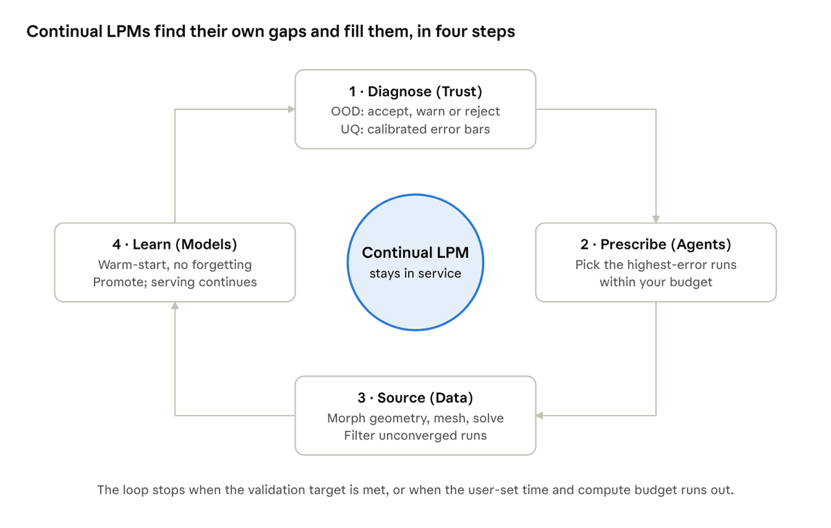
With the Fall 2026 release (generally available in Q1 FY2027), every model built on Luminary ships as a Continual Large Physics Model (CLPM), a model that learns from both new data and its own predictions so that its accuracy and coverage improve over time. Each CLPM runs a four-step loop:
- Diagnose. Out-of-distribution detection scores each input as accept, warn or reject, and uncertainty quantification calibrates the error on every in-distribution prediction.
- Prescribe. Agents use the diagnosis to perform active sampling to select the simulations that will close the largest gaps within the time and compute budget you set, and they stop the loop automatically once the validation target is reached.
- Source. The platform morphs the geometry, meshes it and runs the physics, filtering out malformed or unconverged runs before they reach training.
- Learn. Training warm-starts from the previous weights and folds the new data in without forgetting what the model already knew.
Because agents drive every phase, the model improvement is continual and automatic, while the model stays in service the entire time.
To see how this works in practice, consider a car aerodynamics model built on DrivAerML with a budget of 30 simulations and 5 held-out test designs. The first loop spread 18 simulations evenly across the design space, and each later loop sent its simulations to the regions where the model was least certain:
| Loop | Simulations added | Drag error | Lift error |
|---|---|---|---|
| 0 | 18, spread evenly | 10.4% | 17.1% |
| 1 | 6, where the model was least sure | 4.8% | 7.9% |
| 2 | 6 more, spread apart | 1.6% | 4.0% |
After the second loop, the error fell below the target, and the loop stopped on its own, with every new simulation having gone to the model’s weakest spot.
The same loop also handles designs the model has never seen. Instead of guessing, the model flags the new design, widens the design space to include it, and runs simulations only in the new region. When an engineer proposes new design parameters, the loop scores how much each one overlaps what the model can already represent and spends simulations only on the parameters that are new to it. When the loop is pointed at a goal such as lower drag, the model searches the design space, the solver confirms every candidate, and an engineer makes the final decision.
Versioned models with live updates
A model that keeps learning also has to stay accountable, so every loop saves a new model version, and every version is tested on the same fixed set of held-out cases. You can pin a version to keep its answers stable for a program while the continual model continues to improve alongside it.
Updates also happen without downtime. Predictions continue to be served while the new version is checked, and the new version is promoted only after it passes. Each customer’s improvements stay in their own model, trained on their own data, rather than being folded into a generic release.
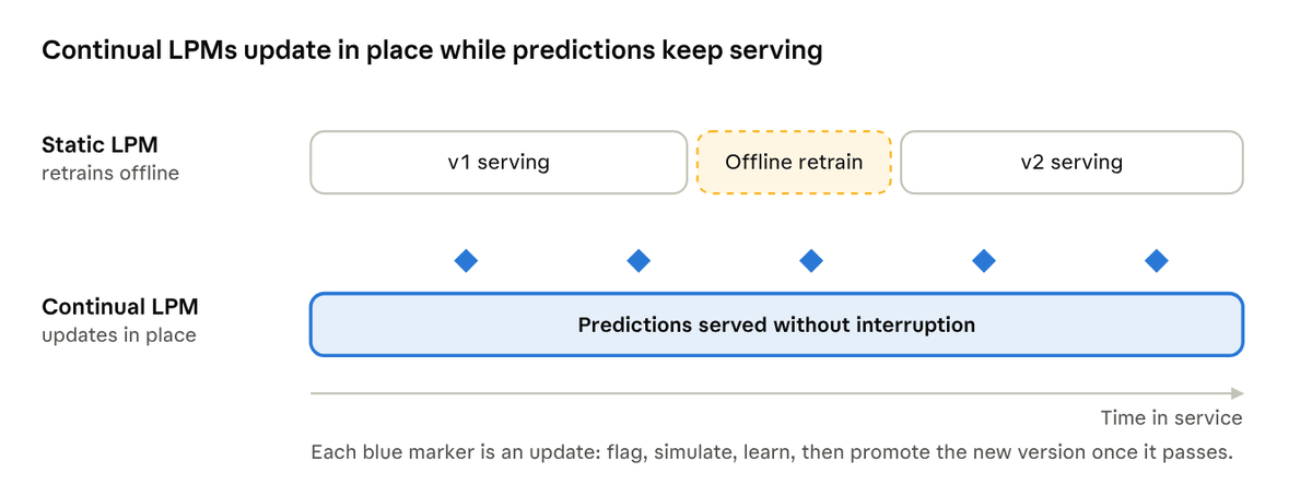
Static vs continual LPM
Agent-led engineering
From one request to a finished workflow
The solver is almost never the bottleneck in a design study. Most of the time goes to the setup and cleanup around the solve, and all of it depends on scarce expertise. With the Fall 2026 release, you describe the task and Luminary Autopilot does the work. Autopilot plans the job, splits it across parallel subagents and runs each step on the platform. Because workflows are durable and run server-side, a job keeps going for as long as the work requires, whether or not you are watching it.
Building a Large Physics Model shows how this comes together. A single agent covers the full lifecycle. It collects simulations across the design space, screens out unconverged runs and physical outliers, and trains the model with Luminary-SMART as the default architecture, configuring inputs, outputs and GPU orchestration for you. It then judges quality with metrics such as R² and MAE, picks the best checkpoint, promotes a model version and returns predictions with their OOD and UQ scores.
Independent workstreams, such as dataset generation, visualization and ensemble analysis, can run side by side in separate sessions, which lets engineers spend their time on the decisions rather than on the steps between them.
Expert agents across the workflow
The Luminary agent puts the distilled knowledge of our R&D staff at your fingertips. Specialized CAD, Data Generation, Training and Visualization agents handle geometry cleanup, defeaturing and parameterization with pre-mesh checks; meshing decisions such as refinement strategy, wall resolution, adaptation and mesh quality; simulation setup, including physics and numerics settings tailored to your application, boundary conditions, motion, outputs and stopping conditions; and Physics AI tasks such as dataset generation, outlier pruning, training, inference and OOD checks.
Here are some example prompts and agent actions:
| You ask | The agent delivers |
|---|---|
| “Can you help parametrize this?” | A parametric model of the geometry, ready to generate a design space, in 27 minutes |
| “Can you help pre-process this geometry?” | Manufacturing CAD turned into simulation-ready geometry in 21 minutes |
| “Can you use this diagram to create a 3D CAD?” | A 3D CAD model from an engineering drawing in 18 minutes |
| “Can you help run these simulations using automotive DDES best practices?” | A full SUV aero campaign set up and run in 29 minutes |
For that last request, the agent built a SnappyHex mesh capped at 200 million cells and checked its cell count, patches and domain size before running a steady SST startup with a moving road and spinning wheels until residuals and drag converged. It then switched to DDES on the same mesh at 0.1 ms steps, discarded 20 flow-throughs of startup, averaged drag and lift over the next 50, and passed the run only if five block means agreed within 1%, before rendering surface pressure for review.
The agent can also stage an entire simulation sequence as a pipeline and explain the methods and settings it chose. In one example, it ran a wall-modeled LES of the LAGOON landing gear at Mach 0.23 and predicted the far-field aeroacoustic noise. Agents work across external aerodynamics, thermal problems, including coupled fluid-thermal analysis, and turbomachinery and internal flows.
Saved workflows
Nobody knows how to do your job better than you, so the agents are built to follow your team’s workflows, standards and specifications. You can perform a workflow once, capture it in a skill or a Python notebook and share it with your team, and you can complement the baseline agent behavior or override it wherever your practice differs. The agent also remembers your preferences across sessions, which turns your team’s conventions into portable automation that anyone on the team can run.
Approval checkpoints
Because black boxes don’t belong in high-stakes engineering, Luminary agents are designed to be transparent, auditable and permissioned. You can see what the agent is doing, and how, while it works; every action leaves a record that you can inspect and review; and irreversible or cost-sensitive actions require your explicit approval.
Agents where you work
You can reach Luminary agents from wherever you already work, including the web UI, the Python SDK, Jupyter notebooks, MCP clients such as VS Code, Cursor and Claude, and Slack and Microsoft Teams.
In Slack, you can mention the agent in a channel or send it a direct message, and because your Slack identity is linked to your Luminary account, the agent works with your permissions. Each thread is its own session that several people can join, any action that changes data or incurs cost waits for approval in the thread, and plots, images and links are posted back where the conversation is happening.
Other systems, including your own agents, can call Luminary agents through the Agents API, and you can choose the language model behind them, from frontier models by Anthropic, OpenAI and Google to hosted models from Google and NVIDIA.
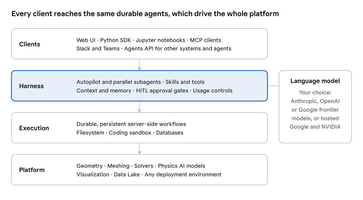
Luminary agent architecture
Data
Physics data is scarce in ways that text and image data are not. Volume is only part of the problem, because training data also has to cover the design space, be trustworthy at the right fidelity, be affordable to generate and store, and be usable once you have it. Addressing all of that takes a platform rather than a single tool, so this release improves every step from geometry to storage.
Geometry generation
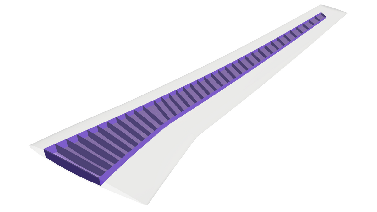
A continual model needs to create new designs on its own rather than wait for someone to draw them, and populating a design space starts with turning one geometry into many. The platform supports both continuous and discrete CAD kernels, geometry repair and modification, and integrations with CAD tools, which gives you several ways to generate variants. You can use a parametric model, as we did when a NASA CRM parametric model in Onshape populated the SHIFT-Wing dataset; you can deform a non-parametric model with morphing-cage parameterization; or you can ask an agent to run geometry preprocessing, repair and parameterization natively in the platform.
Broader physics coverage
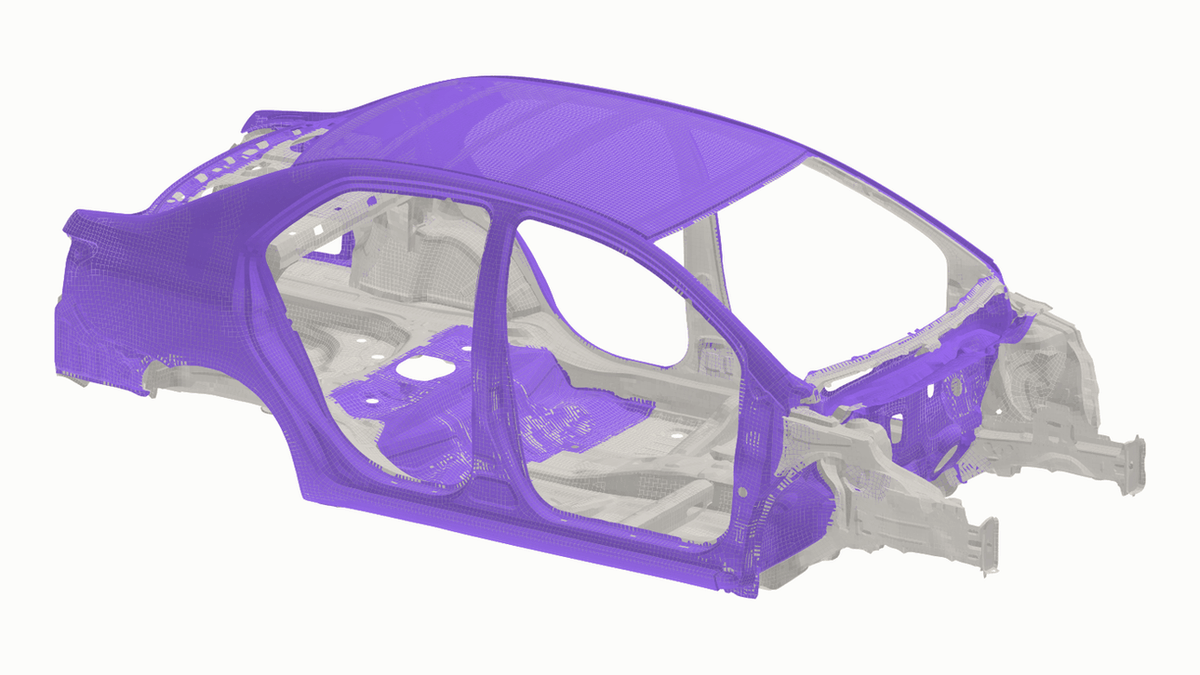
Training data also has to come from the right physics. You can generate it with Luminary’s solvers, bring your own trusted third-party solvers, or bring data you already have, including test data from the real world, as in the DevDay examples that used OpenRadioss for frontal crash and TACS for shell structures. Across these sources, the platform covers the following physics:
| Area | Coverage |
|---|---|
| Fluids and turbulence | RANS, DES, LES |
| Flow regimes | Incompressible, compressible, hypersonic (non-equilibrium) |
| Aeroacoustics | Ffowcs Williams-Hawkings (FWH) |
| Conjugate heat transfer | Coupled fluid and solid thermal |
| Structural mechanics | FEA |
| Motion | Moving reference frame, sliding motion |
Solution-adaptive meshing at scale
Because no one can hand-check thousands of simulations, a trustworthy dataset depends on capturing the physics correctly regardless of who sets up the run. Luminary’s solution-adaptive mesh generation refines the mesh where the flow needs it, for example around the shocks on a NASA C608 configuration between Mach 1.1 and 1.5, and produces results that go beyond what practitioners can achieve by hand. Verification and validation is now open, repeatable and driven by agents, so trust in the solver scales along with the data.
The platform’s scale comes from its CAE roots, starting with GPU-native solvers. Customers run campaigns of thousands of cases today, and one leading space company cut its simulation time from 12 hours to under 10 minutes per run.
Our own SHIFT datasets show what this looks like in practice, with 8 datasets totaling about 56 TB across external aerodynamics, crash and structures. SHIFT-SUV, at 18.3 TB and more than 4,000 samples, and SHIFT-Wing, at 10.2 TB and more than 12,000 samples, together account for 28.5 TB of training-ready data.
Luminary Data Lake
An agent can only work with data it can find, and the same is true for engineers. A design sweep produces hundreds of geometries, meshes and solutions, and they usually end up spread across job folders, storage buckets and laptops.
The Luminary Data Lake gives that data a home on the platform, isolated for each customer. Every object records how it was made, from geometry to mesh to simulation to outputs, and datasets are versioned so that you always know where training data came from. A metadata schema captures what each object contains and how it can be used, which allows application-specific guardrails to streamline workflows, such as only combining solutions with matching fields into a dataset. Indexers generate embeddings, so you can search with filters, ranges and keywords or in plain language, for example “SUV estate variants with high shear on the rear window.”
The Data Lake is wired directly into Luminary Pipelines, which reads Data Lake objects and runs your own transformations and preprocessing as Pipelines stages. Data generated outside Luminary is managed exactly like data generated on the platform, in every deployment, and the Data Lake also hosts reference datasets, including the SHIFT datasets and DrivAerML, so you can train or fine-tune against public baselines alongside your own data.
Models
A Large Physics Model takes geometry and operating conditions and returns physics in seconds, including surface pressure and wall shear, velocity and pressure in the volume, and integrated quantities such as drag, lift and peak temperature. Making that model more intelligent comes down to three things: handling harder physics such as separated flow, wakes, shocks and complex boundary conditions; handling harder geometry, including fine detail and designs nobody has simulated yet; and freeing the model from its dependence on a simulation mesh.
Luminary-SMART updates
Luminary-SMART is mesh-independent by design. Geometry comes in as points sampled from the CAD surface, an encoder compresses millions of points into a few thousand latent points, and a decoder answers for any x, y, z location you ask about, so you encode the geometry once and query as many points as you like without building a simulation mesh.
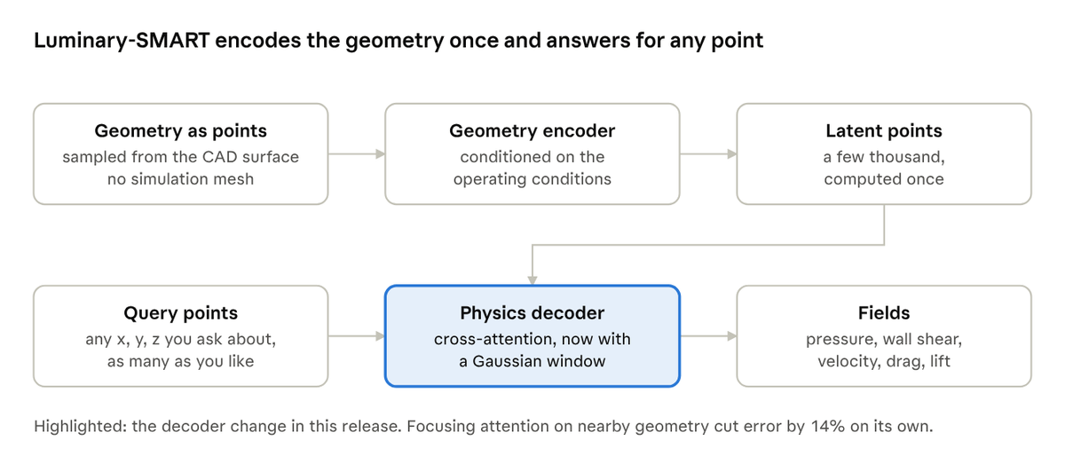
Luminary-SMART architecture
This release ships five model updates. One of them adds a Gaussian window to the decoder that focuses each query point’s attention on nearby geometry, and that change alone cut error by 14%. Together, the updates lowered surface-pressure error on every entry in our benchmark suite, by between 7% and 56%. On DrivAerML, across 50 held-out cars, surface-pressure error fell by 41%, wall-shear error by 44% and drag error by 30%. Because the model size did not change, inference is just as fast, and closer drag predictions on unseen designs mean that more of a design screen can happen before anyone runs CFD.
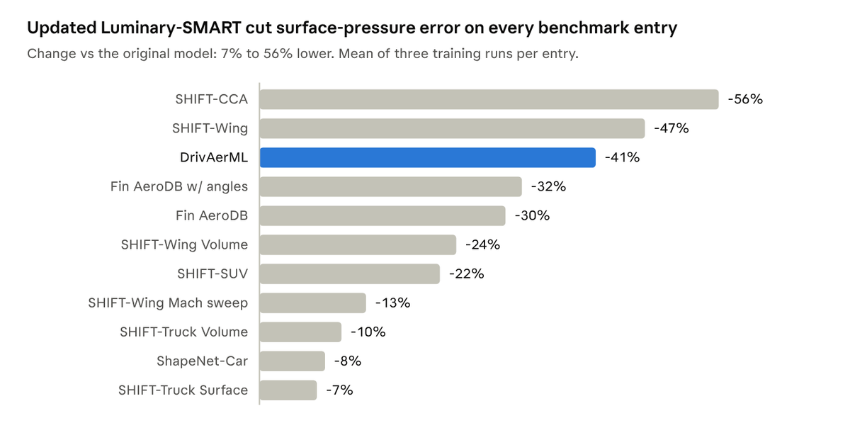
Surface-pressure error change by benchmark entry, 11 entries
Luminary-AB-UPT
Luminary-AB-UPT brings the field’s reference architecture for large automotive simulations onto the platform. Where SMART samples points and attends to latent points, AB-UPT pools neighboring points into supernodes and reads from anchor points on the surface and in the volume, so its cost grows with the number of anchors rather than the number of outputs. The lessons from SMART carried over, and the improved AB-UPT models cut pressure error by between 15% and 45% across the same benchmark entries. Luminary-GeoTransolver and DoMINO also remain available.
D-JEPA (research preview)
Filling an aerodynamic database requires one prediction per cell, multiplied by every design. D-JEPA encodes the geometry once into a compact representation and then swaps in small physics decoders for whatever you need, such as pressure and wall shear, structural displacement, or the design parameters themselves. Its field accuracy is on par with both generative and predictive model families, it was lowest or tied on every integrated force we tested, and it ranked 8 of 8 test designs in the same order as CFD. Adding a structural decoder to a fluid-trained model also required 4.1 times fewer trainable parameters than training from scratch. You can read more in the paper.
Continuous benchmarking
Verification and validation are staples of CAE, and Luminary brings the same rigor to Physics AI by checking every model change in four ways. Each change is verified against held-out simulations with CFD as the reference, it has to show a gain in all three training runs, it has to improve results across the whole evaluation suite rather than a single dataset, and it has to show measurable progress on the industry-relevant tasks in our AI Labs benchmark.
The suite spans automotive aerodynamics with DrivAerML, SHIFT-SUV and SHIFT-Truck; aircraft aerodynamics with HiLiftAeroML, SHIFT-Wing, SHIFT-CCA and an airliner AeroDB; marine, internal flow and heat with the DTC hull, SHIFT-Submarine, SHIFT-Pump, SHIFT-Battery and SHIFT-Electronics; and structures and crash with SHIFT-Crash and SHIFT-NVH. Thousands of training runs, kept and scored the same way, feed better hyperparameters and architecture changes, and every change that passes ships to all customers in the next release, whether they are hosted, on-premises or in their own VPC.
Self-serve training, fine-tuning and continual learning
Model training is now part of the public Luminary SDK, so you, or an agent working on your behalf, can point a training job at a Data Lake dataset and launch distributed GPU training with recommended defaults for the settings that matter most.
Fine-tuning starts from a pre-trained model and adapts it to your domain using either full fine-tuning or LoRA (low-rank adaptation), which trains a small add-on network while the base model stays frozen. In one internal test on DrivAerML, a model fine-tuned from an AeroSUV-pretrained checkpoint reached a best validation loss of 0.104, compared with 0.234 for a model trained from scratch on the same 429 cases.
Continual learning adds new data without catastrophic forgetting, where new training overwrites what the model already knew, by using replay to mix a small sample of the original cases into training on the new data. On an aircraft program, a single continual-learning pass with 48 replay cases cut moment error on a new rudder configuration by a factor of 114, while force error on the original wing stayed at 1.7%. This is the learning step inside every Continual LPM.
Physics-aware learning
A neural network does not know the laws of physics unless you teach them, and Luminary’s physics-aware learning draws on several ways of doing so, including loss-function penalties, imposing some or all of the boundary conditions and fields, constrained optimization, and architectures with built-in structural symmetries.
Model registry
When models keep learning, you need to know which version is serving your predictions. In Model registry, model versions are registered under a parent model, and each version can be promoted, demoted, pinned or retired, with retired versions no longer able to serve inference. Applications that call the parent model pick up a newly promoted version automatically, without any downtime.
Trust
Model Confidence Suite
The usefulness of a Physics AI model depends on knowing when to rely on it. The laws of physics are universal, but a trained model is not, and like most AI it can be confidently wrong. Before an engineer relies on a prediction, two questions need answers: how sure the model is about the question, which out-of-distribution (OOD) detection answers by checking whether the input is close to what the model was trained on, and how sure it is about the answer, which uncertainty quantification (UQ) answers by estimating how large the error is likely to be. With the Fall 2026 release, the Model Confidence Suite answers both questions for every prediction.
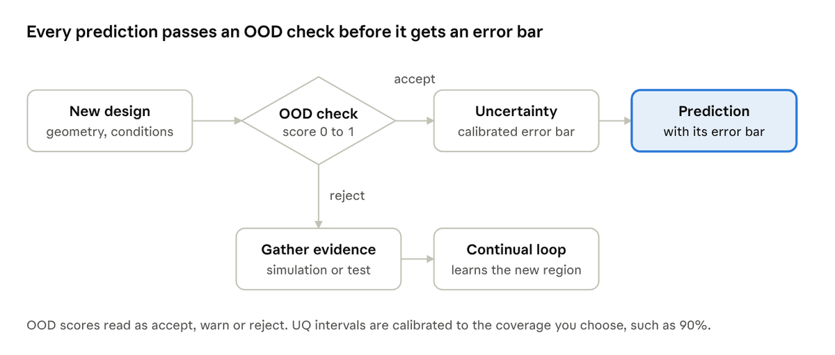
OOD and UQ in sequence
OOD detection runs three checks, on the model’s learned features, on the global parameters and on the geometry’s shape, and it works whether the training data forms one cluster or several. It returns a confidence score from 0 to 1 that reads as accept, warn or reject, so an engineer can tell whether an input sits close to what the model was trained on or far enough outside it that the prediction should not be relied on.
UQ adds an inexpensive error-bar network that runs in parallel with the trained model, learns from the model’s internal features and its errors, and is then calibrated per sample with conformal prediction to give guaranteed coverage. It produces error bars on whole fields as well as on per-sample quantities such as drag. On a transonic wing, field uncertainty estimates reached 90% coverage, with error bars widest at the leading edge, the wing-body junction and the shock, and drag was covered on 68 of 73 unseen in-distribution designs. On a car, field error bars reached 90% coverage and were widest at the grille, hood edge and windshield header, with drag covered on 44 of 50 designs.
The suite has been tested on GeoTransolver, SMART and AB-UPT models across aerospace, automotive and electronics-cooling datasets, and OOD and UQ together add less than 1% compute overhead. They also drive the continual loop, because flagged inputs and wide error bars tell the agent which simulations to run next. You can learn more in our deep dives on OOD detection and uncertainty quantification.
Physics Inference Agent
Teams often discover where a model’s coverage ends only after they have relied on a prediction, and sometimes that discovery happens in a design review. The Physics Inference Agent sits between you and the model to prevent that. You describe your problem in plain English, and the agent turns it into model inputs, picks a model and checks whether that model is valid for the problem. If the input falls outside the training data, the agent tells you and recommends a model that does apply, or a full simulation, and for every result it returns the prediction with its OOD and UQ report and records the model version and inputs that produced it.
V&V solver benchmark catalog
As agents generate training data at scale, the solver behind that data matters even more. The way you build trust in a solver has not changed, since it still rests on verification and validation, but the way the suite is built has: it is now open, repeatable and driven by agents.
The catalog packages Luminary’s evidence in three parts: code verification through the method of manufactured solutions and grid-refinement studies that follow AIAA S-141-2024; solution verification through mesh and timestep convergence, with numerical uncertainty quantified using ASME V&V 20; and validation against public benchmarks such as NASA Turbulence Modeling Resource cases, NAFEMS, DrivAer and DrivAerML, and the AIAA High Lift Prediction Workshop, reported with combined uncertainty. Each entry records the solver version, the dataset snapshot and the date it was last rerun, building on the reports already published at vv.luminary.ai.
Running and analyzing results
Batch inference
A trained model delivers the most value when it can answer thousands of questions at once, such as the predictions across a full flight envelope that an aerodynamic database requires. With the Fall 2026 release, a single API call can submit N cases, which also makes batch inference a single step for an agent. In our Q3 test, a 1,000-case batch finished in about 5 minutes, with each case a 500,000-triangle STL run through a Luminary-SMART model of about 12.5 million parameters. Results are stored as artifacts that you can download and query. We deliberately optimized for throughput over single-case latency, because volume work such as AeroDB generation matters more to our customers than round-trip time.
Agents that answer program-level questions
Once predictions take seconds, agents can run a model thousands or even tens of thousands of times to answer the questions a program actually asks, from design through maintenance:
| Stage | Question | Method |
|---|---|---|
| Design | Which design is best? | Optimization |
| Certification | How does the aircraft behave across its flight envelope? | Envelope characterization |
| Manufacturing | How does as-built variation change performance? | Uncertainty quantification |
| Operation | What is the aircraft doing now, given its sensors? | Data assimilation |
| Maintenance | What caused that reading, and when will the part fail? | Inverse problems |
Visualization and Analysis Agent
Post-processing is repetitive work, because it means opening one case after another to check the same surfaces and probe the same lines. The Visualization and Analysis Agent now runs long analyses across many pipeline runs or inference results at once, with skills for debugging failed simulations, extracting features, and identifying and grouping surfaces. Its outputs are reusable analysis artifacts, so the next batch gets the same treatment, and Autopilot can call the agent as one step in a larger workflow.
Agent-first interface components
An agent can run your simulation, but you still need to see the geometry, the mesh and the result before you approve the next step. The platform interface is now built from modular views of geometries, meshes, simulations, inference results, comparisons and datasets, which agents assemble into an interface for the task at hand so that the evidence for an approval appears right next to the request. New interactive widgets add slices, streamlines and isosurfaces.
Deployment
Same platform, every environment
Every capability in this release runs on the same platform wherever you deploy it, whether that is SaaS, your own VPC, a private cloud, a fully air-gapped environment or a hybrid setup. Each customer’s model and data stay in their own environment, and the data remains exportable.
Agents are also available in export-controlled environments. In ITAR deployments, all model traffic runs through approved regional endpoints, outbound traffic is denied by default, and tools that need outside network access, such as web search, are turned off, while SDK code generation and notebooks work as they do in commercial deployments within documented ITAR data-handling limits.
Conclusions
A static model stays fixed until someone retrains it. A Continual Large Physics Model finds its own gaps, fills them and learns on its own, and with the Fall 2026 release, agents run that loop. Engineers set the goal, see every action and make the decisions, and the agents do the rest.
These capabilities premiered at Physics AI DevDay 2026 on November 17, 2026, with sessions on data generation, model architectures, trustworthy Physics AI, agentic automation and Continual Large Physics Models. Register here.
Getting started
There are several ways to get started with the Fall 2026 release:
- Read the Luminary SDK documentation to learn about training, fine-tuning and batch inference.
- Connect your coding agent to the platform through the Luminary MCP server.
- Try predictions from a SHIFT-Wing model in the public Physics AI demo.
- Talk to our field engineering team about your first use case.