Introducing SHIFT-NVH: A Large Physics Model for Body Vibration and Gauge Design

In an automotive program, once the body geometry is frozen, sheet gauge and material are the main design variables left for noise, vibration and harshness (NVH). Each proposed gauge change needs a modal and forced-response solve on the full-body finite element (FE) model to show how the body modes and road-induced vibration move, part by part. Gauge, material and vehicle speed multiply the candidates faster than an NVH team can solve them before gauges are released. Suppliers often do not have the full-body model, and when OEMs release it, it frequently needs rework to run in the supplier’s toolchain.

A Large Physics Model (LPM) is a neural network trained on solver output that predicts the full solution field for a new design without running the solver. SHIFT-NVH is an LPM trained on FE solves of one body-in-white. It takes the gauges of 15 parts, the material and the vehicle speed as inputs. It returns RMS acceleration in x, y and z at all 130,713 surface nodes under ISO 8608 class B road excitation. Engineers can evaluate gauge and material changes, and see which parts each change affects, without the FE model, which stays with whoever generated the training data. On 192 held-out cases, the median relative L2 field error is 1.1%.

Dataset

Body and design space

We used the 2010 Toyota Yaris body-in-white from the public NCAC crash model. It has 213 parts and 130,713 nodes. We selected 15 parts that a supplier could plausibly re-gauge, including the roof, both side panels, the firewall tray and the rear floor.

Each part’s gauge varied by up to ±30% of nominal. We sampled 100 designs plus the baseline with a Latin hypercube. The mesh is identical across all designs. Only shell thickness and material properties change.

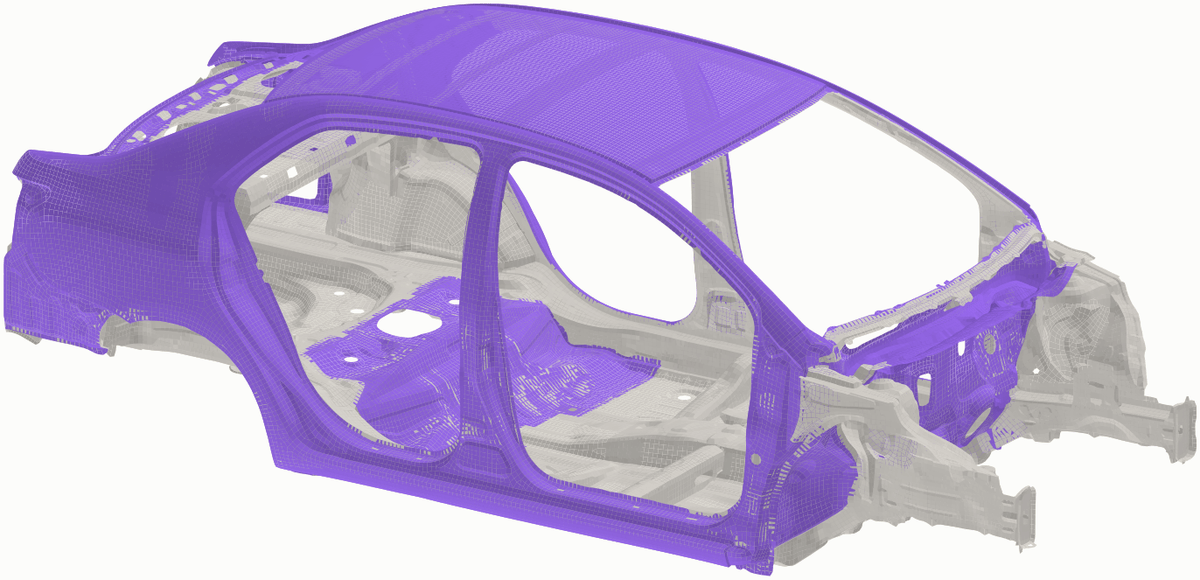
Figure 1. The 2010 Toyota Yaris body-in-white from the public NCAC crash model. The 15 parts whose gauge varies are shown in purple.

We repeated every design in aluminium and magnesium. We scaled each gauge by (E_steel / E)^(1/3) to hold plate bending stiffness constant. That gives factors of ×1.43 for aluminium and ×1.64 for magnesium.

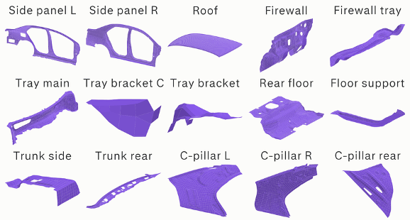
Figure 2. The 15 parts whose gauge varies in the design study.

Modal solves

We ran free-free modal solves for all 303 bodies. Each solve returns 6 rigid-body modes and the first 14 elastic modes. On the steel baseline the elastic modes span 18 to 56 Hz. Modes 1 and 2 are global body modes. The steel baseline also has a local mode concentrated on the firewall tray at 25.6 Hz, which Figure 3 omits.

Video. Mode 1 of the steel baseline at 18.3 Hz. Color shows displacement magnitude.

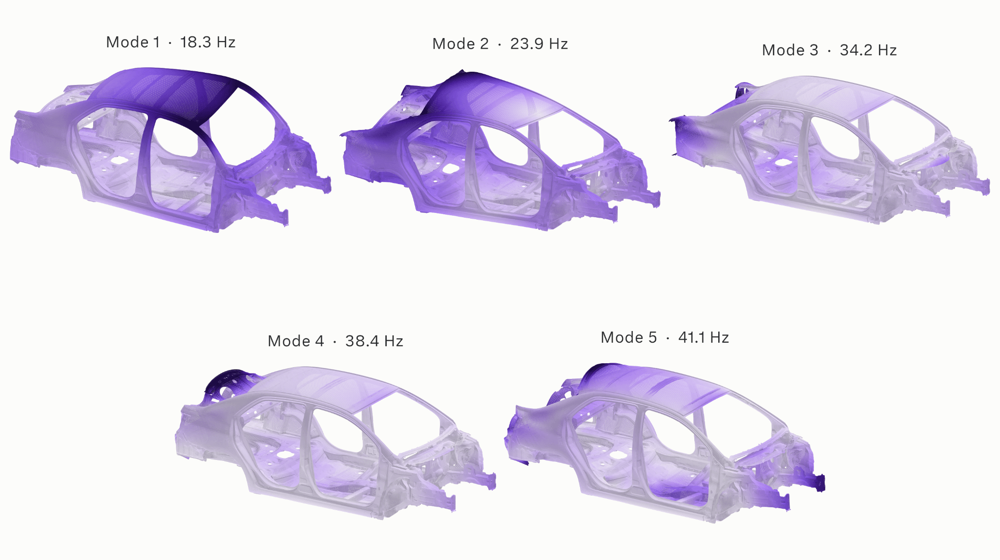
Figure 3. Five elastic modes of the steel baseline. Modes 1 and 2 are global. The local firewall-tray mode at 25.6 Hz is not shown.

Gauge changes can reorder or mix modes, so sorting by frequency compares different shapes across designs. We tracked each mode to the baseline with a mass-weighted modal assurance criterion (MAC):

MAC(a, b) = |aᵀMb|² / ((aᵀMa)(bᵀMb))

Here a and b are mode shapes and M is the mass matrix. The unweighted MAC omits M and can misidentify modes on a body with strongly non-uniform mass distribution.

Road excitation

Road input enters the body at 8 attachment points taken from the crash model. These are the front strut tops, rear spring seats, rear damper tops and rear torsion-beam pivots. We modeled each corner as a quarter-car. Spring rate (18.5 N/mm) and damper rate (1.93 N·s/mm) come from the crash model. Unsprung mass and tire rate are assumed values.

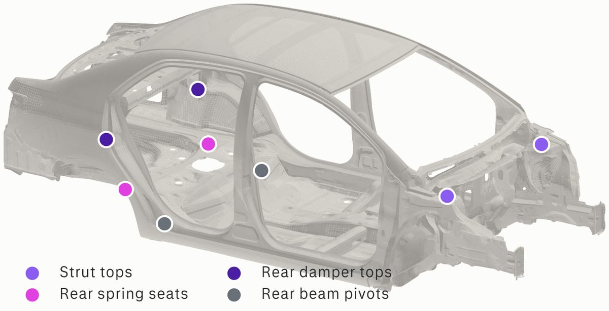
Figure 4. The eight body attachment points used for road input.

The road profile is ISO 8608 class B. The rear wheels see the front profile delayed by wheelbase divided by speed. Left and right tracks are partially correlated. We computed the elastic response by modal superposition with 1.6% modal damping. We ran each body at 30, 50, 80 and 110 km/h, giving 1,212 road cases.

Effect of gauge and material on the body

Frequency response

Small frequency shifts produce large changes in the FRF near lightly damped resonances. Across the 100 designs, the FRF at a given frequency between 15 and 45 Hz spans a median of 14 dB. Material shifts every peak up, because the lighter bodies carry the same bending stiffness with less mass. The spread from gauge is similar across the three materials.

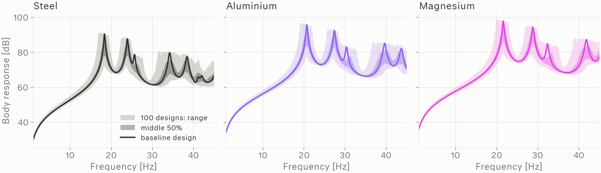
Figure 5. Body FRF across the 100 gauge designs for each material: full range, middle 50% and baseline.

Road response

At 50 km/h, a gauge change moves part-averaged RMS acceleration by a median of 4.7% and by 24% at the 95th percentile. In 47% of part-cases the change is 5% or more. The firewall tray bracket has the largest mean change across the design space.

Material has a larger effect than gauge. Body-in-white mass is 233 to 253 kg in steel, 114 to 124 kg in aluminium and 86 to 93 kg in magnesium. At equal bending stiffness, the lighter bodies show higher body RMS acceleration on the same road.

Body RMS acceleration generally rises with speed. The steel body is an exception, with lower vibration at 110 km/h than at 80 km/h. Mode 2 (23.9 Hz) is excited by front and rear inputs in antiphase. At 110 km/h the wheelbase delay puts the rear input in phase with the front at 23.9 Hz. The net excitation of mode 2 then largely cancels.

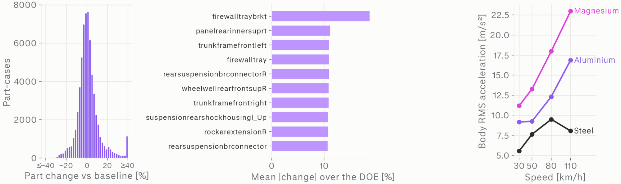
Figure 6. Left: part RMS change against the baseline at 50 km/h. Center: parts with the largest mean change. Right: body RMS acceleration against speed by material.

Model

Luminary-SMART is Luminary’s encoder-decoder architecture for LPMs. It maps a set of design parameters to a field on the surface mesh.

The SHIFT-NVH road model takes 19 inputs: the 15 gauges, the material properties (Young’s modulus E, density ρ and Poisson’s ratio ν) and the vehicle speed. It outputs RMS acceleration in x, y and z at each of the 130,713 nodes. Part-level vibration is the node average over each part. One model covers all three materials and all four speeds.

Because the mesh is fixed, the model does not learn geometry variation. It learns how thickness and material redistribute the response over a known mesh.

We split the 1,212 cases by design: 840 for training, 180 for validation and 192 for testing. The training set fits the model weights. The validation set selects the saved model. The test set is used only for the results below. All four speeds and three materials of a given design fall in the same split. Every test design is therefore unseen in any material or speed. We trained on 4 NVIDIA H100 GPUs for 300 epochs, where an epoch is one pass over the training set. The best validation error was 0.020 in relative L2.

Results on held-out designs

Field and part accuracy

Relative L2 error is the L2 norm of the prediction error over all nodes, divided by the L2 norm of the reference field. The reference is the modal forced-response solution described above.

Metric (n = 192 test cases)	Result
Field relative L2 error, median / worst	1.1% / 2.6%
Part RMS error, median / p95	0.47% / 2.4%
R² of predicted vs. reference change against baseline	0.974
Change error, p95	2.7 percentage points
Correct sign, parts changing by ≥ 5%	99.5%
Parts flagged as changed, precision / recall	95% / 94%
Overlap of the top 10 most-affected parts, mean	8.5 of 10

The test cases span 16 unseen designs, 3 materials and 4 speeds, across all 213 parts. A part counts as changed when its RMS acceleration moves by 5% or more from the baseline. Precision is the fraction of predicted changes that are real, and recall is the fraction of real changes the model predicts. The median part RMS error (0.47%) is about one tenth of the median gauge-induced change (5.4%). This ratio is what lets the model separate a real gauge effect from prediction error at the part level.

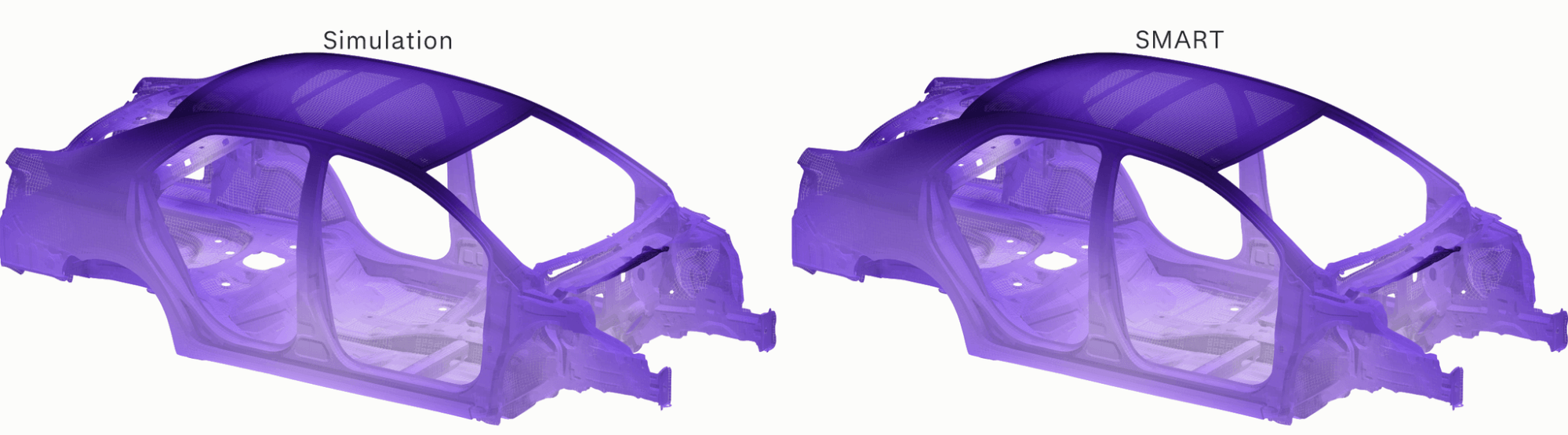
Figure 7. RMS acceleration on an unseen aluminium design at 50 km/h. Left: simulation. Right: SHIFT-NVH. Same color scale.

Mode shapes

We trained a second SMART model on the steel modal data. It takes the 15 gauges as input and predicts the 5 elastic mode shapes shown in Figure 3. On 16 unseen steel designs, mean MAC against the reference is 0.98 to 1.00 for modes 1 to 4 and 0.92 for mode 5. This model does not predict frequencies.

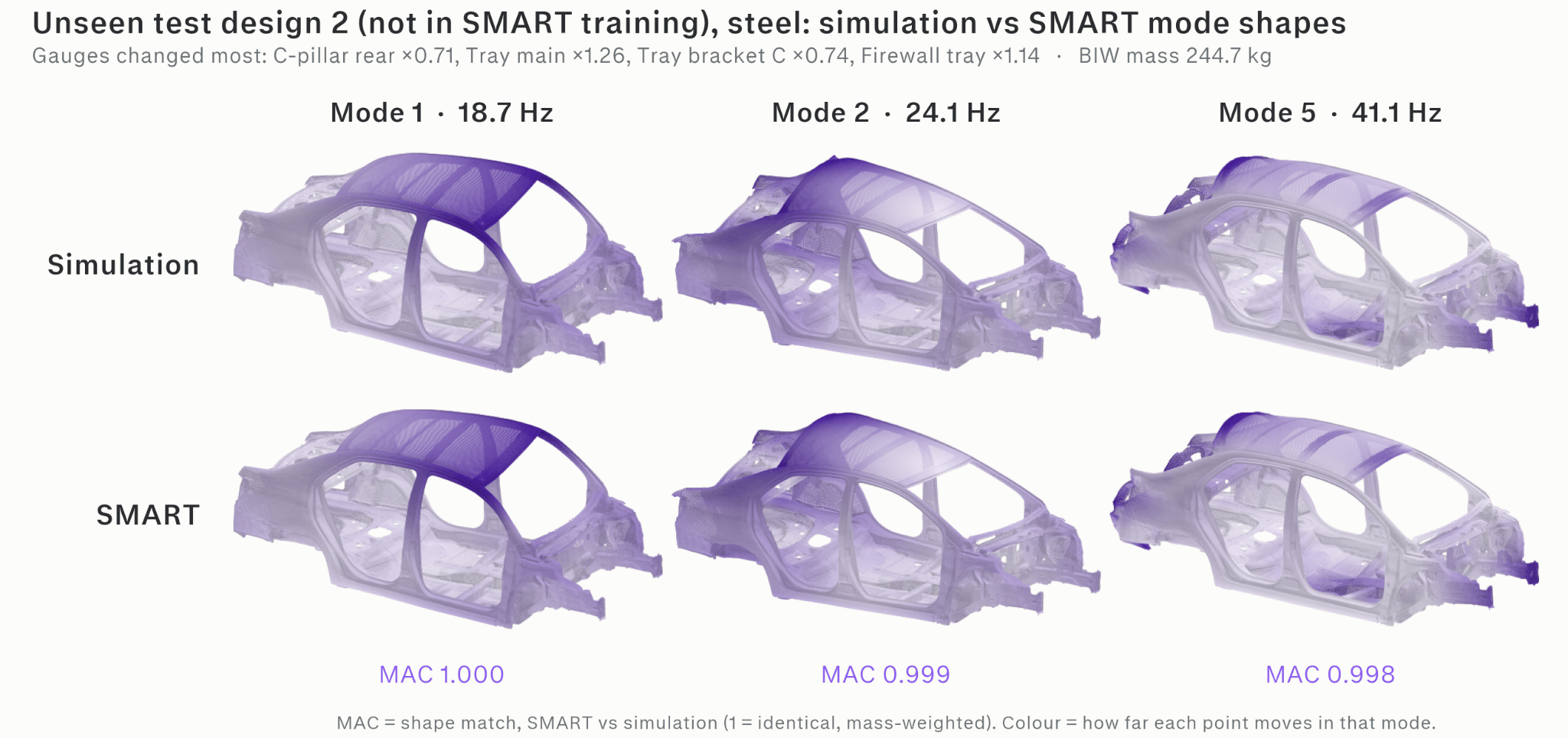
Figure 8. Modes 1, 2 and 5 on an unseen steel design. Top: simulation. Bottom: SHIFT-NVH mode-shape model.

Applications

Looking ahead

SHIFT-NVH answers the late-program gauge question without a full-body solve for each candidate. It predicts road-induced vibration at every node from part gauges, material and vehicle speed. On held-out designs, the median part error is 0.47%, about one tenth of the median gauge-induced change of 5.4%. Differences between designs therefore remain visible at the part level.

The current model covers one body-in-white with a fixed mesh. Its range is ±30% gauge on 15 parts, three materials, four speeds from 30 to 110 km/h and an ISO 8608 class B road. Within that range, engineers can screen gauge and material combinations with the model. Full FE and physical testing remain the basis for final gauge decisions on the shortlisted designs.

Try it

SHIFT-NVH joins Luminary’s SHIFT family of Large Physics Models, alongside SHIFT-Crash, SHIFT-Truck and SHIFT-Battery. Try the SHIFT-NVH demo to see how the body’s mode shapes and frequencies change with panel gauges and material. To see SHIFT-NVH on your own body-in-white, or to request a technical walkthrough, talk to our team.