Many engineering quantities of interest depend on how two or more physical fields interact with each other. A wing in flight twists and bends under aerodynamic load, and the deformation changes the load. Thermal–structural problems in turbine blades and electronics packages couple in the same way. A coupled analysis exchanges results between the solvers for each field and iterates until they agree.
For example, in a typical engineering organization, the aerodynamics team runs CFD and the structures team runs finite element analysis, often in separate groups. Every iteration of a coupled analysis crosses that boundary. The structures engineer requests a flow solution for the current shape, and the aerodynamics engineer meshes, sets up and runs it. Each request can take a long time to come back.
The tools are also hard to connect. A solution from one solver has to be exported to the other, mapped onto its mesh and applied as a load. The deformed shape often has to be remeshed before the next solve. Automating that chain is a project of its own, and the most expensive solver still runs at every iteration.
In practice, engineers often skip coupled analysis in early design. The interaction then shows up late, as costly rework, or the design ends up suboptimal.
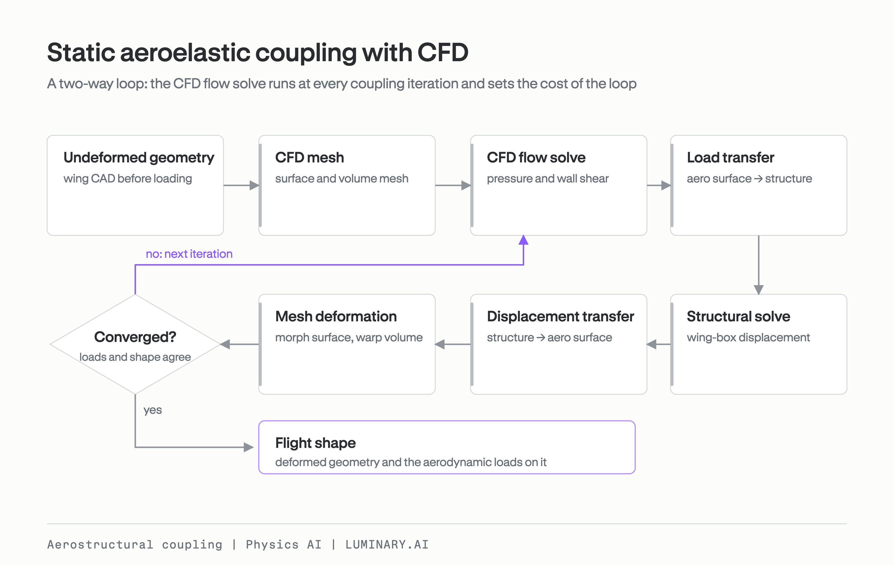
Figure 1. Static aeroelastic coupling with CFD. The CFD flow solve runs at every coupling iteration and sets the cost of the loop.
What Physics AI changes
A large physics model (LPM) is a Physics AI model trained on solver data. It predicts full output fields, such as surface pressure or structural displacement, directly from CAD geometry and operating conditions. By predicting the fields a high-fidelity solver would return, and by skipping the workflow steps that coupling two solvers requires, LPMs address both problems above.
The first is the distance between experts. The aerodynamics team can train and validate a flow LPM and hand it to the structures team, who then run it whenever their analysis needs new loads. The same pattern applies outside aerostructures: a designer can query an LPM trained on CFD without waiting on a CFD specialist.
The second is the toolchain. An LPM goes from CAD to a solution in seconds. This reduces case setup and the steps needed to move results from one toolchain to another.
Coupling also needs full fields. A structure responds to the spanwise and chordwise distribution of the load, which a model that predicts only scalars such as total lift or root bending moment cannot supply. LPMs predict the whole surface field, so they can sit inside a coupled loop in place of a solver.
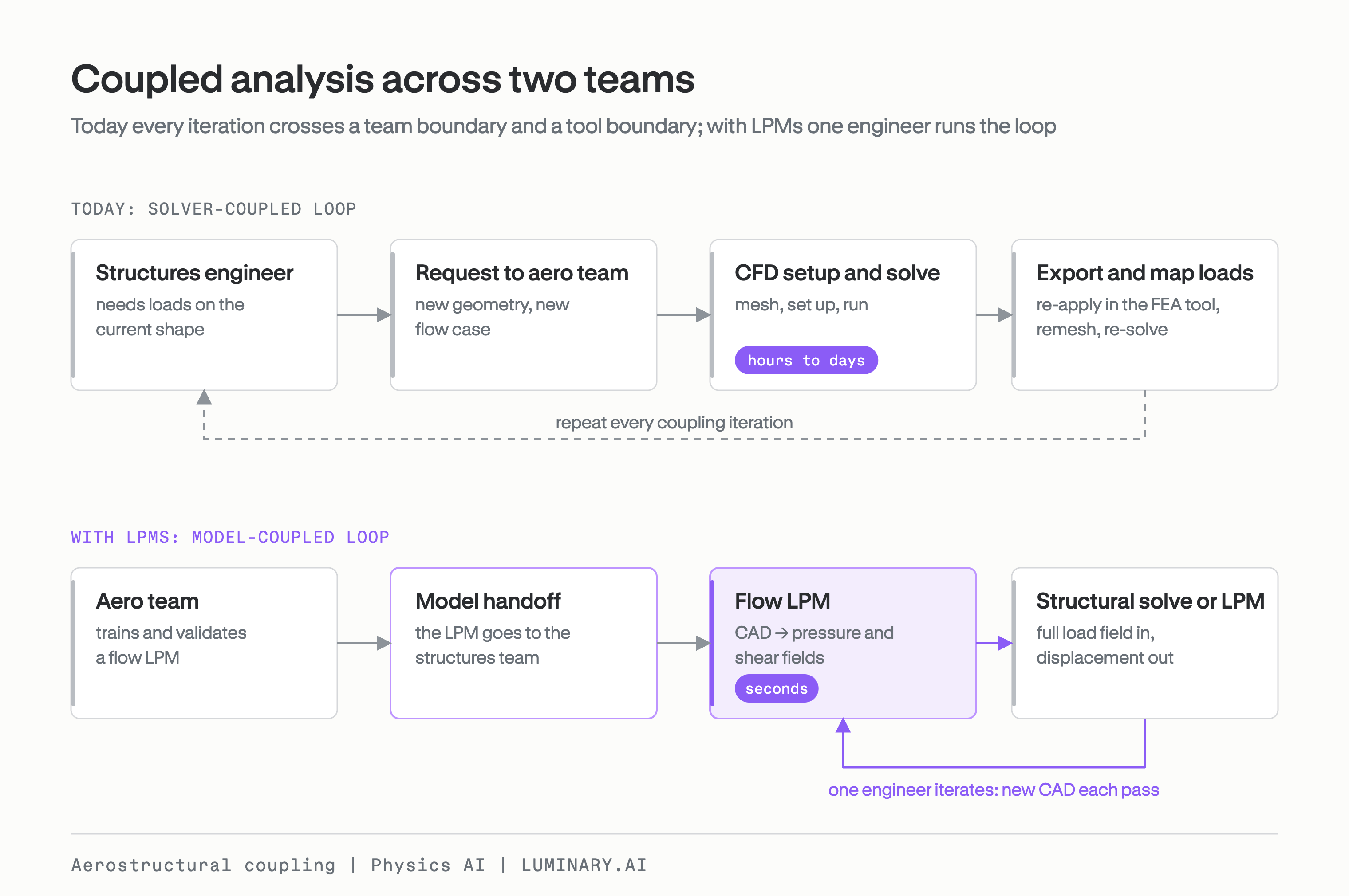
Figure 2. Coupled analysis across two teams. Today each iteration crosses a team and a tool boundary; with LPMs one engineer runs the loop.
The result is a coupled workflow that one engineer can run in minutes. The loop is faster, and it also changes who can run the analysis and how often they can run it.
The demonstration: a transonic swept wing
We demonstrated LPM coupling on the static aerostructural response of a transonic swept wing. In flight, the wing twists under load. In a sweptback wing, the twist usually reduces the local angle of attack as one moves from the wing root toward the tip (a phenomenon called washout), leading to a loss in actual lift relative to a rigid simulation. Washout can also alter the real effectiveness of control surface deflections. In this example, we demonstrate washout and the resulting loss of lift on the SHIFT-Wing geometry, and model aeroelastic twist as the main geometric quantity that changes from one coupling iteration to the next. We ignore bending as a second-order effect, but the same analysis can easily be extended to include flight conditions and the associated bending deformations when they are nontrivial.
The loop passes aerodynamic loads to a shell model of the wing box, which returns the deformation back to the wing geometry. With CFD on three NVIDIA H100 GPUs, using mesh adaptation, a converged loop took an average of four hours to complete.
We ran the demonstration in two steps. Step 1 replaces CFD with a flow LPM and keeps the structural solver. This is the setup for a structures engineer who wants to keep their own solver and take loads from an aerodynamic model the aerodynamics team has signed off on. Step 2 replaces the structural solver with a second LPM, so two LPMs exchange full fields at every iteration.
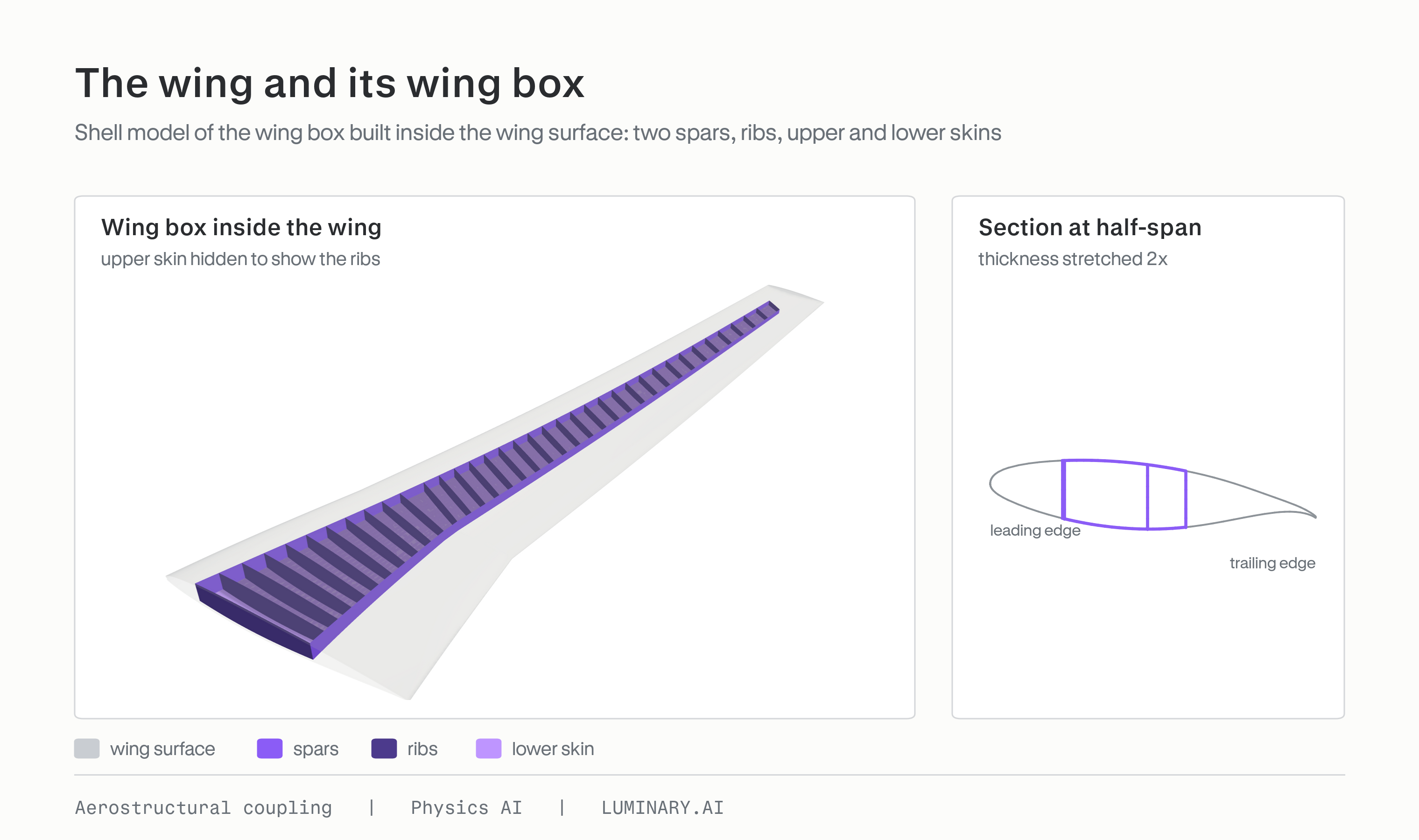
Figure 3. The wing and its wing box: shell model of the wing box inside the wing surface, with a section at half-span.
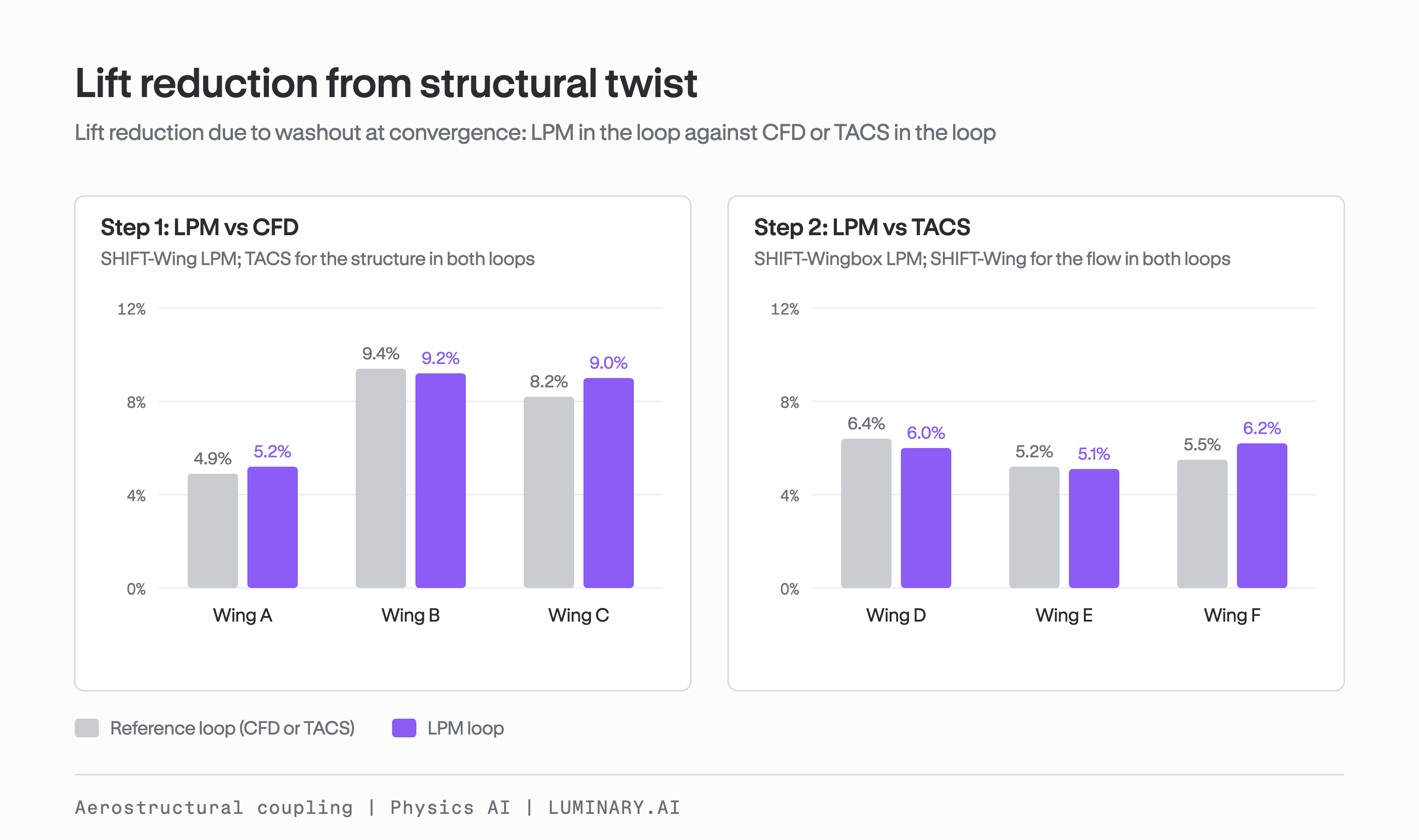
Figure 4. Lift reduction due to washout at convergence on six wings. For Wings A–C, the reference is CFD + TACS and the LPM loop is SHIFT-Wing + TACS. For Wings D–F, the reference is SHIFT-Wing + TACS and the LPM loop is SHIFT-Wing + SHIFT-Wingbox.
Step 1: an LPM coupled to a structural solver
SHIFT-Wing is built on Luminary-SMART and predicts pressure and wall shear stress on the wing surface. The training data for this work is a subset of the SHIFT-Wing dataset.
We solved the structure with TACS [1], an open-source finite element solver, on a shell model of the wing box. The skin and spar thicknesses are fixed across cases and vary along the span, with values derived from Gray et al. [3] and Kenway et al. [4]. Loads and displacements are exchanged between the wing surface and the wing box through MELD [2], a conservative load and displacement transfer scheme.
Each iteration runs SHIFT-Wing, transfers the loads, solves the structure with TACS and converts the displacement to a new wing CAD. No step involves meshing. A converged loop took 8 to 11 minutes on one NVIDIA T4 GPU, against an average runtime of about 4 hours for the CFD loop on three H100 GPUs. That is more than 20 times faster, on one smaller consumer-grade GPU.
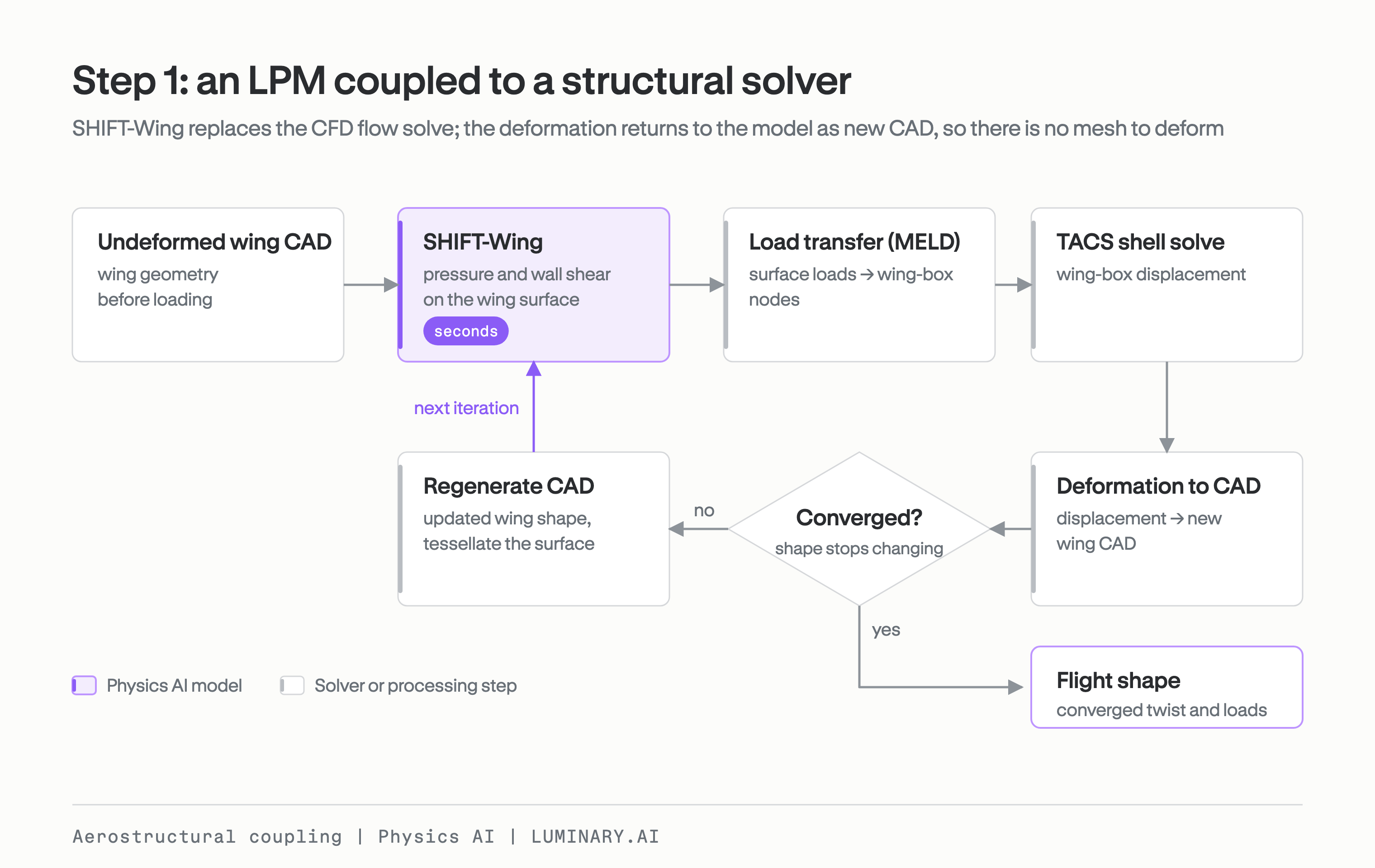
Figure 5. Step 1: SHIFT-Wing coupled to a TACS shell solve through MELD. The deformation returns to the model as new CAD.
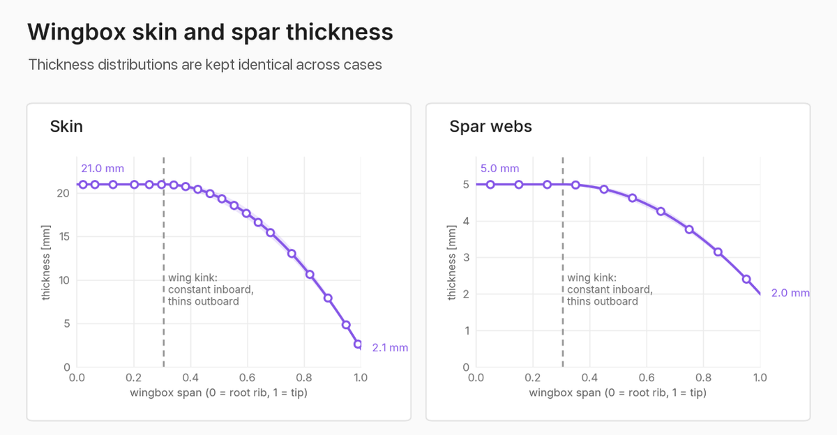
Figure 6. Wing-box skin and spar thickness distributions along the span. The same distributions are used for every case.
We ran three wing geometries through both loops. Both loops converged in four iterations on every wing, and the lift reduction they predicted differed by 0.2 to 0.8 percentage points.
| Wing | CFD loop: undeformed → converged | Lift reduction | SHIFT-Wing loop: undeformed → converged | Lift reduction |
|---|---|---|---|---|
| A | 908 → 864 kN | 4.9% | 923 → 875 kN | 5.2% |
| B | 973 → 881 kN | 9.4% | 984 → 893 kN | 9.2% |
| C | 435 → 400 kN | 8.2% | 442 → 402 kN | 9.0% |
Most of the difference in absolute lift is already present at the undeformed shape, before any coupling. It comes from SHIFT-Wing’s prediction error on each geometry, between about 1% and 2% of the undeformed lift.
The twist shows how much the geometry changes at each iteration. The tip rotates 0.8° to 1.5° nose down at convergence, and about two thirds of that rotation happens in the first iteration. At every iteration, the tip twist in the SHIFT-Wing loop is within 0.04° of the CFD loop.
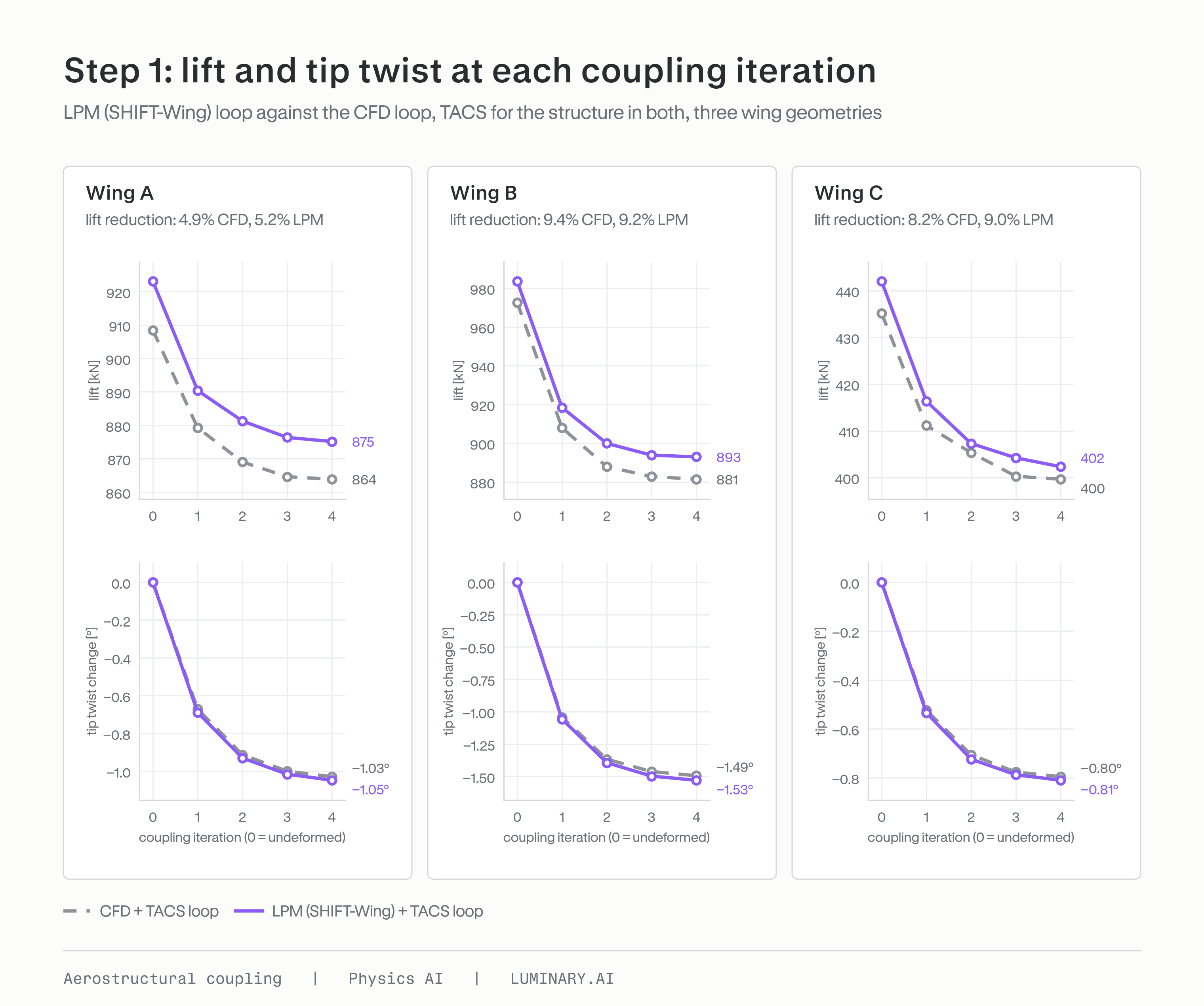
Figure 7. Step 1: lift and tip twist at each coupling iteration, LPM (SHIFT-Wing) loop against the CFD loop on three wing geometries.
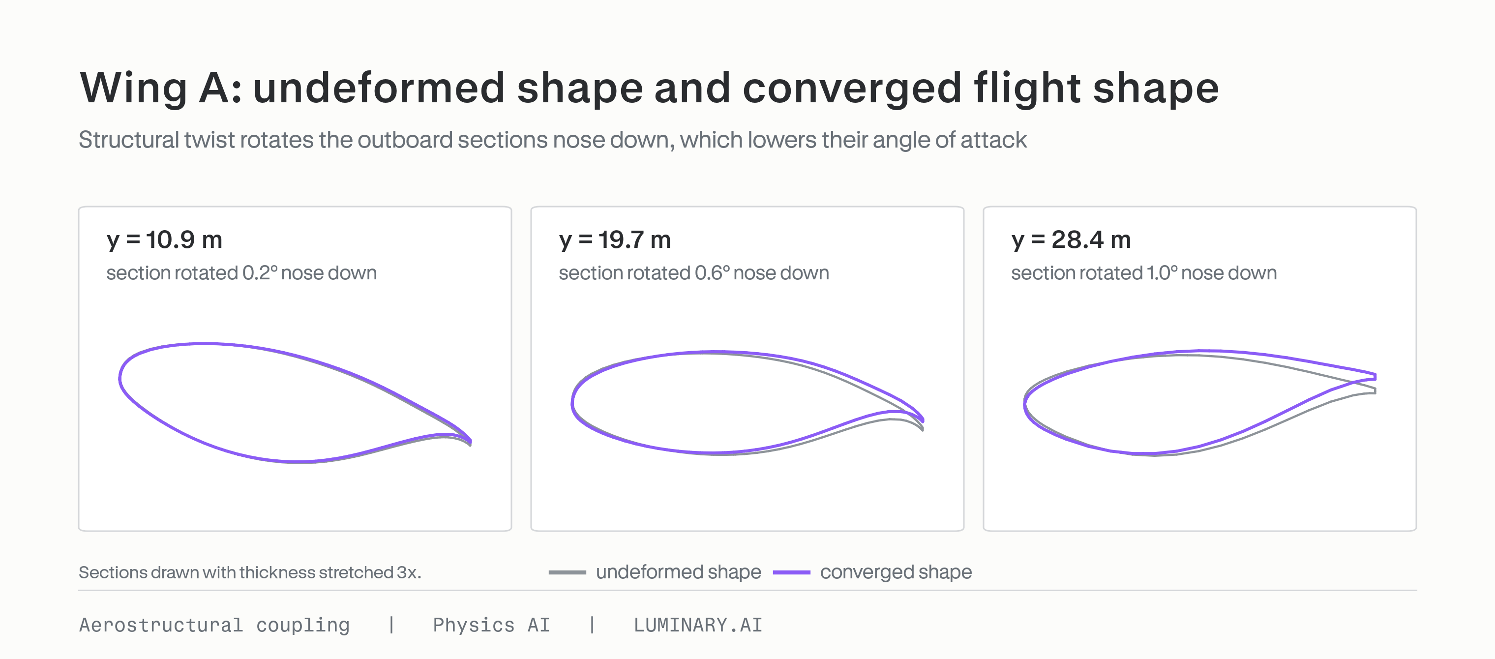
Figure 8. Wing A: sections of the undeformed shape and the converged flight shape. Outboard sections rotate nose down.
Step 2: two LPMs in one loop
SHIFT-Wingbox predicts the displacement and stress field on the wing box from the wing surface and the pressure and wall shear stress on it. It uses a modified version of the Luminary-SMART architecture that takes both the geometry and the surface fields on it as input. This lets the model map aerodynamic fields to structural solutions across a range of wing shapes and flight conditions. We trained it on about 1,400 TACS solutions, with loads taken from different SHIFT-Wing configurations.
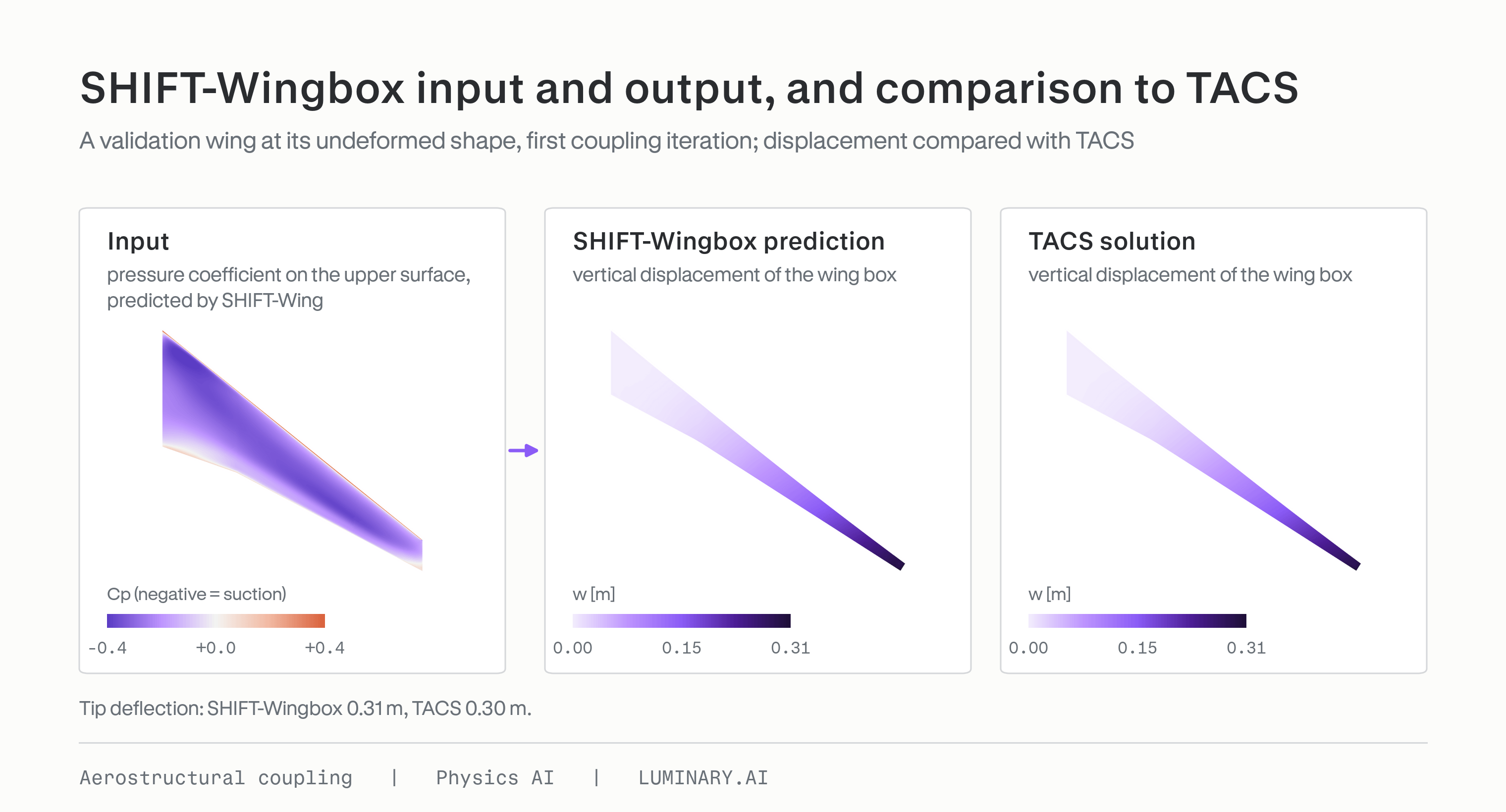
Figure 9. SHIFT-Wingbox input and output, and comparison to TACS.
The rest of the loop is unchanged from step 1. Both loops in this step use SHIFT-Wing for the aerodynamics, so the comparison measures SHIFT-Wingbox against TACS.
We show three converged solutions from the test set of this workflow. The tip twists agree closely: the converged values are within 0.04° of each other, on about 1° of nose-down twist. At convergence, the lift reduction due to washout from the two loops agrees to within 1 percentage point.
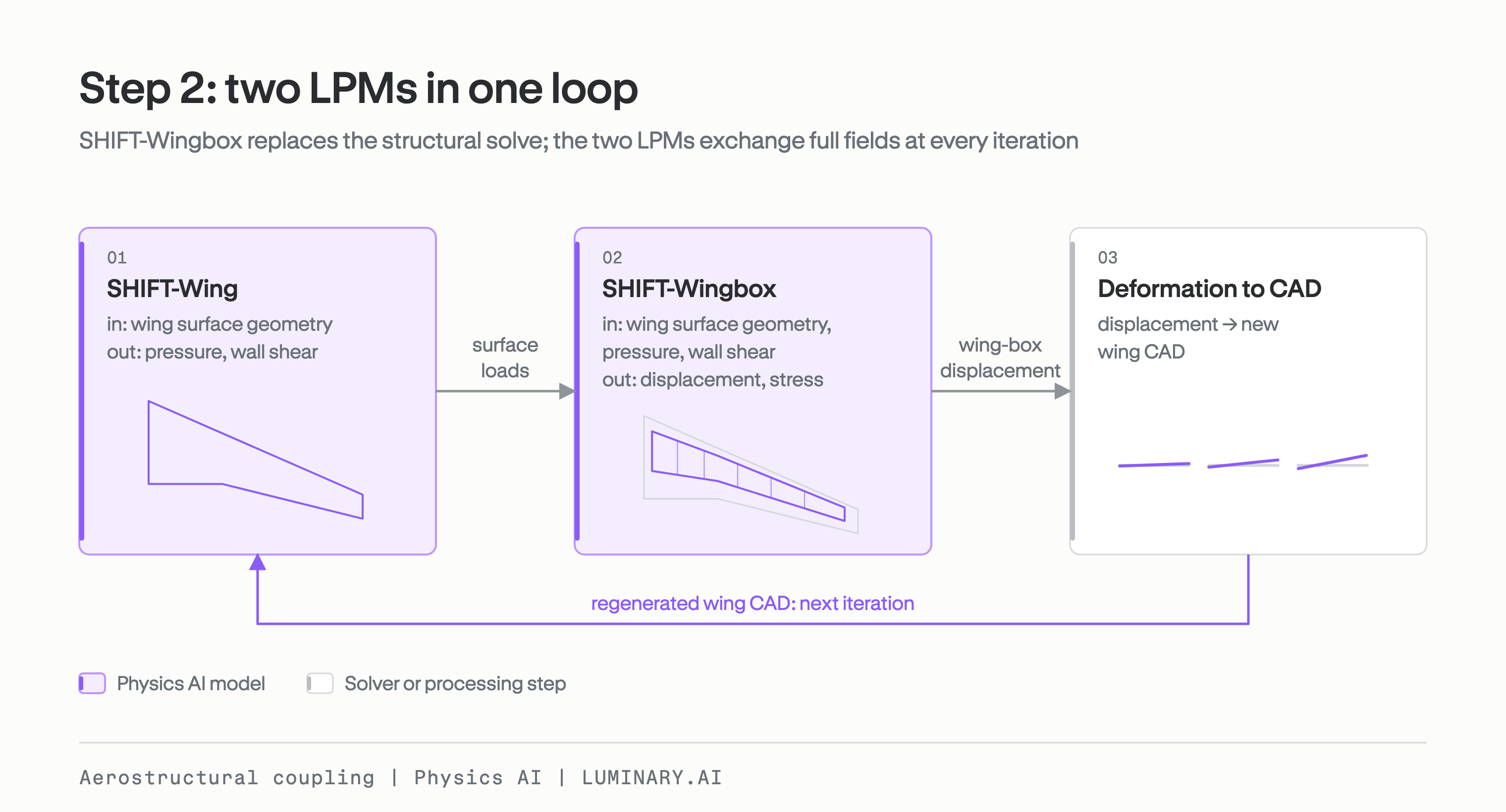
Figure 10. Step 2: SHIFT-Wing and SHIFT-Wingbox exchange full-field solutions at every iteration.
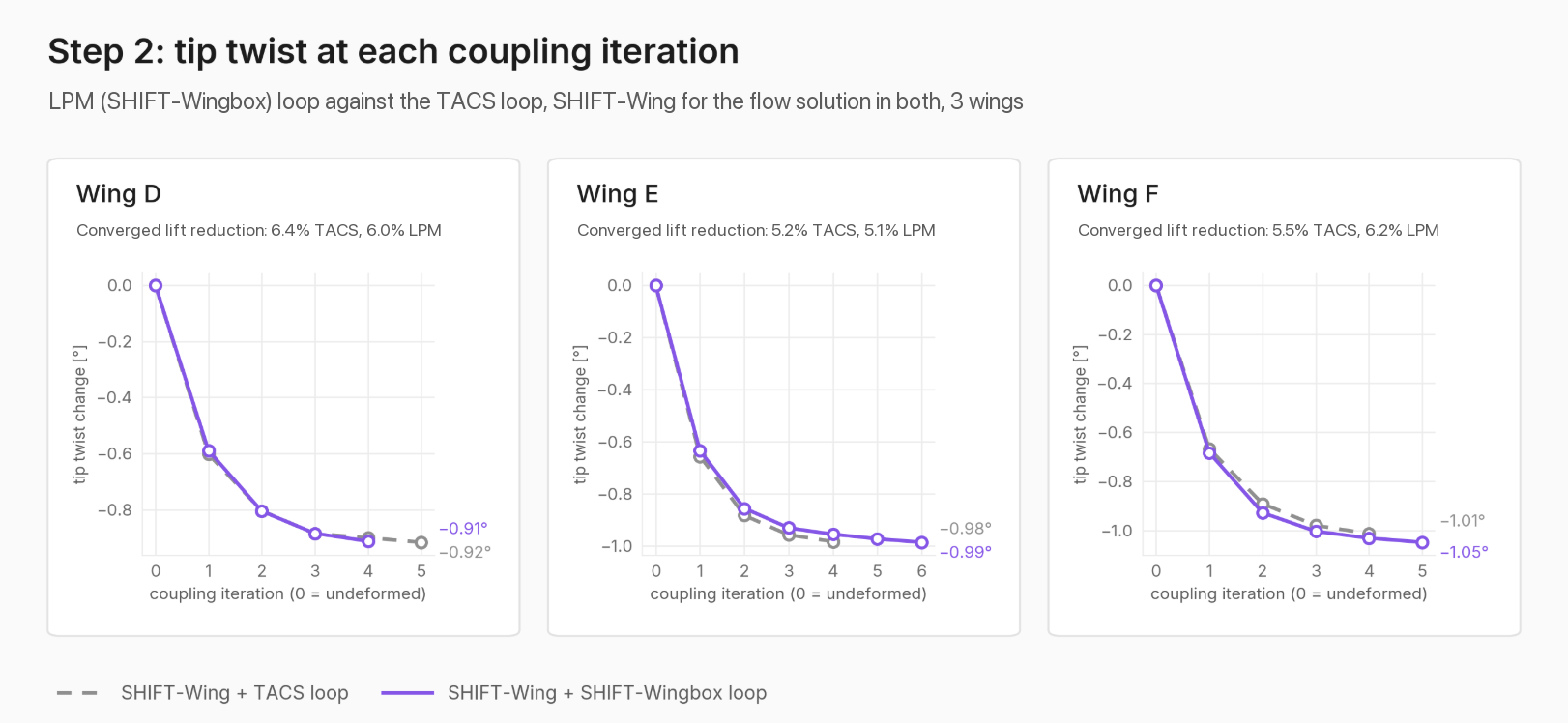
Figure 11. Step 2: tip twist at each coupling iteration, LPM (SHIFT-Wingbox) loop against the TACS loop, with SHIFT-Wing for the flow solution in both.
Summary
Coupled analysis is held back by the cost of the participating high-fidelity solvers, the siloed nature of disciplinary teams in large organizations and the complexity of coupling toolchains between them. LPMs that predict full fields from CAD address all three bottlenecks. On a transonic swept wing, a flow LPM coupled to a structural solver converged in 8 to 11 minutes against about 4 hours for CFD, with the predicted lift reduction due to washout agreeing within 0.8 percentage points on three geometries. We also developed a modified version of Luminary-SMART that accepts full field solutions on CAD and tested it in a coupled analysis with SHIFT-Wing. Two LPMs coupled together predicted lift reduction due to washout within 1 percentage point and tip twist within 0.04° of the loop with the structural solver, on three geometries.
References
[1] Graeme J. Kennedy, Joaquim R.R.A. Martins, “A parallel finite-element framework for large-scale gradient-based design optimization of high-performance structures,” Finite Elements in Analysis and Design, Volume 87, 2014, Pages 56–73.
[2] Kiviaho, Jan F., and Graeme J. Kennedy. “Efficient and robust load and displacement transfer scheme using weighted least squares.” AIAA Journal 57.5 (2019): 2237–2243.
[3] Gray, A. C., Martins, J. R. R. A., Volle, F. A., Burke, B. J., Engelstad, S. P., and Kennedy, G. J., “Comparisons of Results for a High-fidelity Aeroelastic Optimization Benchmark Problem,” AIAA SciTech 2026 Forum, Orlando, FL, AIAA 2026-0762, Jan. 2026.
[4] Kenway, G. K. W., Kennedy, G. J., and Martins, J. R. R. A., “Aerostructural Optimization of the Common Research Model Configuration,” 15th AIAA/ISSMO Multidisciplinary Analysis and Optimization Conference, Atlanta, GA, AIAA 2014-3274, June 2014.