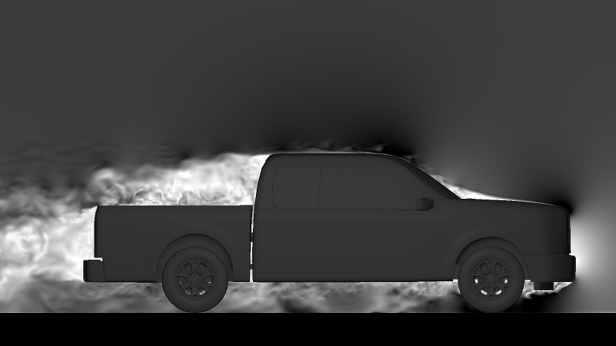
Vocabulary of Physics AI

Vocabulary is one of the biggest barriers to entry into any technical domain, and the barrier is highest where conventions are still forming. Physics AI is rooted in the same math and physics as simulation, but because it pulls together several fields at once, familiar concepts can read as alien. An epoch in model training sounds new; it plays much the same role as an iteration in a solver run. Few terms are pure rebrands, and the differences carry real engineering weight, but learning the analogies between what you already know and what is new is the fastest way to build intuition for the technology.

The analogies only stretch so far. A latent space describes a nonlinear, non-orthogonal, case-dependent manifold. Attention is a learned, data-dependent aggregation with no built-in conservation guarantee. In ML practice, validation means monitoring a held-out dataset during training; in CAE simulation, validation means checking physical accuracy against experimental evidence.

For an engineer who already builds CAE simulation models, the parallels run deep. This page maps the core vocabulary to the six stages of model development: the terms you will encounter, what they mean, and where you can draw analogies to CFD and FEM.

Physics AI is the general approach: replacing repeated high-fidelity simulation with a learned function trained on simulation data. A Large Physics Model is what that approach produces: a single trained model that covers a design space wide enough to stand in for many individual simulations, sharing the same relationship a large language model has to many individual language tasks. The six stages below describe how to build a Large Physics Model.

The core mental model

Most Physics AI models approximate a single learned function:

f_θ(p, G, ξ) ≈ u(p, G, ξ)

where G is the geometry, ξ contains operating conditions, p is a spatial query coordinate, u is the physical quantity at that location, and θ represents the learned model weights. For external aerodynamics:

geometry + freestream conditions + query coordinate
↓
learned surrogate
↓
pressure, velocity, or wall shear at that point

The table below is a quick translation layer.

Traditional CAE	Closest Physics AI concept	Contrast
Reduced Order Model (ROM) evaluation	Inference	The learned map can predict the entire field or values at any given coordinates.
Proper Orthogonal Decomposition or reduced-basis coordinates	Latent representation	Usually nonlinear, case-dependent, non-orthogonal, and not energy-ranked
Shape functions / interpolation weights	Attention or learned aggregation	Weights are data-dependent and learned; they do not satisfy consistency or conservation automatically
FEM/FVM stencil	Graph neighborhood or learned stencil	The neighborhood may be geometric rather than topological, and may be randomly sampled
V&V validation	Test metrics, Out Of Distribution evaluation, physical checks	Statistical test error is a prerequisite for V&V; completing V&V requires separate physical checks

The Large Physics Model (LPM) development lifecycle

↻ Stages 02 through 05 are rarely a single pass. In practice they iterate as data coverage expands, architectures are refined, and validation reveals gaps.

Stages 1 through 3 primarily reuse vocabulary from Design Of Experiments (DoE) campaigns or solver-database projects. However, the vocabulary shift becomes more pronounced in stage 4, where model architecture introduces terms without direct CAE equivalents. These terms resurface in stages 5 and 6, where familiar words like validation and latency acquire new meanings within the context of an ML process.

Stage 1: Design space and operating space parameterization

The first question in any Physics AI program is identical to the first question in a design of experiments campaign: which parameters vary, over what range, and with what distribution? The ML vocabulary that surrounds this question is mostly statistical, but the engineering stakes are the same.

Design Space. A design space defined by varying geometry, loads, material parameters, boundary conditions, or operating conditions. An LPM learns a single map valid across the entire family. Traditional simulation solves each instance individually.

Sampling strategy. The rule that determines which parameter combinations are used in simulations is crucial. Three variants are particularly important: uniform sampling assigns equal probability to all domain points, which is simple but inefficient near the boundaries of physical validity. Importance sampling concentrates the sampling density in regions that are expected to be physically complex, such as near transonic conditions or flow separation. Area-weighted sampling, which is applied to surface queries, draws points proportional to the physical area, ensuring that small, high-curvature facets do not dominate the training distribution.

Data augmentation. Creating additional training samples through transformations: reflections, rotations, coordinate jitter, or parameter interpolation. For aerodynamics, mirroring a configuration across a plane of symmetry doubles the effective dataset at no simulation cost. Augmentation is only valid when the transformation is a true physical symmetry and leaves the governing equations unchanged.

Stage 2: High-fidelity simulation at scale

The simulation database sets the accuracy ceiling for everything downstream. Errors in training data propagate into the learned model and cannot be corrected later. What is new here relative to a single simulation project is scale: convergence and setup consistency now need to be checked automatically across thousands of cases, including the edge cases at the boundary of the design space. Reviewing each case one at a time no longer scales.

Training case. One complete simulation: a geometry, its operating parameters, and the resulting physical field. The model will be exposed to thousands of these during training.

Conditioning parameters. The operating and physical quantities supplied to the model alongside the query coordinate, the ξ in the function notation above: for external aerodynamics, Mach number and angle of attack; for structural problems, material thickness, load direction, and boundary condition flags.

Target. The quantity the model is trained to predict. Pressure coefficient, velocity components, wall shear stress, displacement, stress tensor components, and integrated forces are all common targets depending on the application.

Ground truth. The reference target values, typically produced by a high-fidelity solver. Solver output carries discretization error, iterative convergence error, turbulence-model error, and constitutive-model error. A Physics AI model trained on RANS predictions inherits those errors along with the RANS coverage of operating regimes.

Normalization and nondimensionalization. Neural network normalization, scaling inputs to zero mean and unit variance, is a numerical training device. Physical nondimensionalization, using chord length, freestream dynamic pressure, or elastic modulus as reference quantities, carries physical similarity information. The two serve different purposes. Nondimensionalized inputs tend to produce mappings that transfer more reliably across Reynolds or Mach number ranges because the similarity structure is encoded in the input representation.

Preprocessing. Transformations applied before training: coordinate normalization, unit conversion, field scaling, or removal of cells where numerical artifacts dominate. Decisions made here affect what the model can learn from the data.

Stage 3: Data curation and management

A well-curated dataset is harder to build than it sounds. The splits, normalization choices, and geometry representations made at this stage determine what the model can and cannot generalize.

Training, validation, and test sets. The standard three-way split: the training set updates model weights; the validation set guides hyperparameter choices, architecture decisions, and stopping criteria; the test set provides the final evaluation and is kept out of reach until all model decisions are complete.

Parametrically related cases, for example variants of the same baseline geometry at different Mach numbers, must be split carefully. A model that sees Mach 0.7 of a geometry during training and Mach 0.8 in the test set is being evaluated on interpolation inside a known family.

Geometry point cloud. An unordered set of 3D points representing the geometry surface, carrying coordinates, normals, area weights, curvature, or material labels. It is generally much cheaper to generate than a solver-quality volume mesh and is the standard geometry representation for mesh-independent Physics AI models.

Signed distance function (SDF). A scalar field giving the distance to the nearest surface boundary, with sign indicating interior or exterior. It gives the model explicit boundary-proximity information that raw coordinates alone do not carry, which matters for predicting boundary-layer behavior and near-wall quantities.

Mesh-independent and mesh-sampling-sensitive surrogates. A mesh-independent surrogate does not require the solver-optimized volume mesh as a structural input at inference. It may still require a CAD-derived surface mesh or point cloud. A mesh-sampling-sensitive surrogate’s internal representation is tied to mesh topology, density, or connectivity, which introduces mesh bias: the model may exploit correlations from adaptive refinement, for example boundary-layer clustering that implicitly signals shock or separation locations, and then degrade on a different mesh.

Stage 4: Model training

Surrogate model. A fast approximation to a high-fidelity solver or experiment. The category includes polynomial response surfaces, Gaussian processes, reduced-order models, neural fields, neural operators, and learned time-steppers.

Field surrogate. A surrogate that predicts a spatially distributed field, such as pressure, velocity, temperature, displacement, or stress, at every point in the domain. This is the dominant form in modern Physics AI.

Neural operator. A neural architecture intended to approximate an operator between function spaces: for example, the map from boundary conditions and geometry to the resulting PDE solution field.

Encoder and decoder. An encoder transforms geometry, point-cloud, field, and parameter inputs into an internal representation. A decoder transforms that latent information and query coordinates into physical outputs.

Latent space. The internal lower-dimensional or structured representation used by the model. The closest CAE concept is a reduced coordinate space, but a latent space is typically nonlinear, non-orthogonal, not energy-ranked, and changes with the input case. Individual latent dimensions rarely carry interpretable physical meaning.

Attention. A learned, data-dependent weighted aggregation. In transformer-based Physics AI models, attention allows a query point to draw information from distant geometry or physical-state tokens in a single operation, without the sequential depth that graph message-passing would require. Attention weights are learned computational quantities; they are not automatically conservative, consistent, or symmetric.

Loss function. The scalar objective minimized during training. Common choices include mean squared error, relative L2 error (field error normalized by field magnitude), area-weighted surface error for surface quantities, and composite losses that combine multiple physical quantities with tuned weights. The relative L2 formulation, ||prediction - truth||₂ / ||truth||₂, normalizes out field magnitude and makes errors comparable across different physical quantities and operating conditions.

Physics-informed loss. The PDE residual evaluated at the model’s field predictions, added to the training objective alongside the data-fit term. Directly analogous to the convergence residual in an iterative solver: it measures how well the learned field satisfies the governing equations at a sampled set of collocation points. A data-only loss measures fit to observations; a physics-informed term measures equation satisfaction. The two are not equivalent and both can be nonzero independently.

Overfitting. Low training error combined with poor performance on unseen cases. The model has memorized training geometry-field pairs without learning the underlying physical mapping. Overfitting is addressed through regularization, data augmentation, and early stopping before the training loss diverges from the validation loss.

Stage 5: Validation

In-distribution performance. A test case drawn from the same distribution as the training data, a geometry from the same family, the same operating range, the same mesh type, provides a measure of how well the model learned the training distribution. Good in-distribution performance is necessary but not sufficient for engineering use.

Out-of-distribution (OOD) generalization. OOD shifts come in distinct forms: new geometry families or topology, new operating regimes (subsonic to transonic, elastic to plastic), new mesh or query-point distributions, and new physical phenomena absent from training. A model can generalize across new geometries in a familiar regime while failing at regime shifts, or the reverse. Each shift type requires its own evaluation.

Verification and V&V validation. In CAE simulation, verification asks whether the computational model solves the intended equations correctly; validation asks whether the model represents real physical behavior accurately enough for the intended use. In ML practice, validation typically means monitoring a held-out set during training. Statistical test accuracy is a prerequisite for starting engineering V&V. Completing V&V requires separate physical checks against experimental evidence.

Uncertainty quantification. Estimating prediction uncertainty from limited training data, noisy targets, model ambiguity, or OOD inputs. Without uncertainty estimates, there is no reliable signal that a prediction falls outside the model’s competence region. Deploying a model without uncertainty bounds in high-consequence engineering is the same as deploying a solver without a convergence criterion.

Stage 6: Deployment and inference

Inference latency. Wall-clock time for one prediction request. Interactive design tools require sub-second response. Batch screening campaigns care more about throughput than per-case latency.

Query independence. The prediction at one spatial coordinate is unchanged by the presence, order, or batching of other query coordinates. Formally: f(p | G, ξ) = f(p | G, ξ, P) for any set of other query points P. Query independence lets a large domain be evaluated in arbitrary spatial chunks without altering pointwise results, which is what enables scalable inference on million-point geometries without approximation.

Chunked inference. Evaluating a large query set in smaller batches to fit within GPU memory. The results are exact when the model has query independence and approximate otherwise. Architectures that apply self-attention across all query points violate query independence by construction.

To see these concepts applied to a real architecture, read Luminary-SMART: The New State of the Art Model Architecture for Large Physics Models. It covers mesh dependence as a learned shortcut, benchmarking beyond training metrics, and the architectural choices that make query independence and chunked inference work at scale.