Uncertainty Quantification for Large Physics Models

In Quantifying the Unknown, we split trust in a Large Physics Model (LPM) into two questions. The first asks whether an input resembles the data the model was trained on. Out-of-distribution (OOD) detection answers that question, and that post showed how we score an input before the LPM runs. The second asks how far a prediction for an in-distribution input is likely to sit from the true value. Uncertainty quantification (UQ) answers the second question, and it is the subject of this post.

UQ attaches an error bar to each prediction at every point in the output, calibrated to contain the CFD value at a coverage the user chooses. This post uses 90%, and the same method gives 80%, 95% or any other level. An LPM predicts the surface fields on a new design in minutes, where a CFD run takes hours. A wrong prediction looks the same as a right one, and every decision that uses the prediction depends on how far it can be trusted. Four uses show what UQ adds:

• Design screening. When a dozen designs finish within 1% of the best drag, error bars separate the designs that are clearly better from the ones tied within the model’s accuracy.
• Peak local loads. The upper end of a per-point error bar bounds the local pressure on a panel such as a side window or a sunroof. An integrated drag or lift value carries no local information.
• Reading the flow. Per-point error bars show which regions of the surface, such as a mirror wake or a shock, need a targeted CFD check.
• Optimization. A candidate whose predicted gain is smaller than its error bar can be set aside before it reaches CFD or a prototype. The widest error bars also show where the next simulation adds the most information.

How we quantify uncertainty

Existing methods and their limits

Two methods from the deep-learning literature are the usual starting points. A deep ensemble trains several copies of the model, typically five, from different random starts and reads uncertainty from how much the copies disagree. Monte Carlo (MC) dropout keeps dropout switched on at inference and repeats the prediction many times, typically about fifty, with a different random subset of the network switched off each time.

Both methods have three problems for an LPM on a full-vehicle mesh. They multiply the cost of training, inference or both. They cannot be added to a model that is already trained: MC dropout needs dropout layers in the architecture from the start, and a deep ensemble trains each member with an extra output that predicts its own variance. They also do not produce a calibrated error bar. The spread across copies measures how much the predictions disagree with each other. Copies trained on the same data with the same architecture can share a blind spot and agree on the same wrong answer, so their error bars still need rescaling against held-out simulations.

	Training time	Inference time	Added to a trained model	Calibrated
Single LPM, no UQ	10 hours	10 seconds	n/a	n/a
Deep ensemble (5 members)	~50 hours	~50 seconds	No	No
MC dropout (~50 passes)	10 hours, retrained with dropout	~10 minutes	No	No
Luminary UQ	10 hours + 10 minutes on one T4 GPU	~10 seconds + one small-network pass	Yes	Yes

The rows use illustrative round numbers for an LPM that takes 10 hours to train and 10 seconds per prediction. The 10-minute companion-network training time is measured.

Our approach

We leave the trained LPM unchanged and add a small companion network. The network learns how large the LPM’s error tends to be at each surface point. It reads three inputs: the LPM’s internal description of the local flow at that point, a summary of the whole geometry, and the prediction itself. It outputs the size of the error bar for each field.

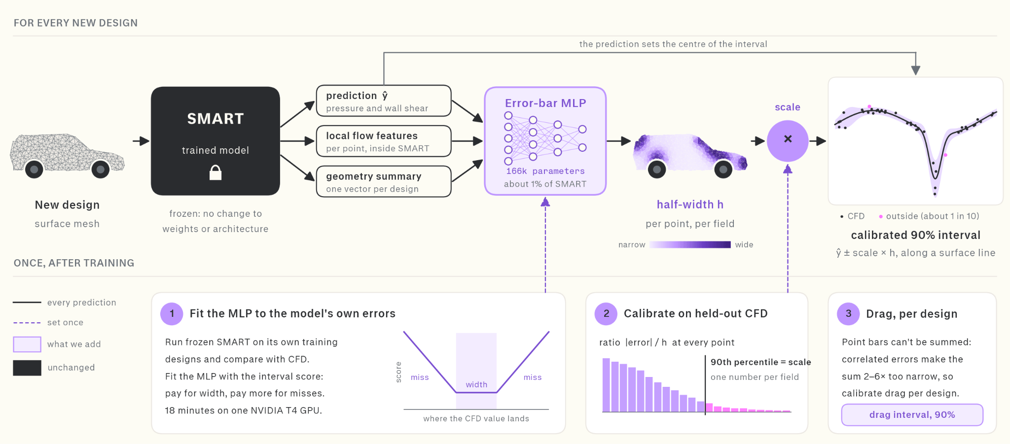
Figure 1. UQ on a trained LPM. The error-bar network reads the LPM’s prediction, per-point flow features and a geometry summary. It is fitted once to the LPM’s own errors, then calibrated on held-out CFD, with drag calibrated separately per design.

We train the companion network on the LPM’s errors on its own training designs. The loss is an interval score, which charges for every unit of error-bar width and charges more for every miss. Its optimum is the error bar that just contains 90% of the errors. Like multi-fidelity correction models [1], the network learns from the gap between a cheap prediction and CFD. It learns the size of that gap, without its sign.

An LPM’s errors on its training designs are smaller than its errors on new designs, so we calibrate the error bars on held-out simulations the LPM never saw. This step uses normalized split conformal prediction [2, 3], a calibration method that reaches a stated coverage without assuming a shape for the error distribution.

Integrated quantities are calibrated separately.

Advantages

• Works on a pre-trained model. UQ is added to an LPM after training, including a model the user brings. The LPM’s architecture, weights and training are unchanged.
• Small. The companion network has about 166,000 parameters, roughly 1% of the LPM, and trains in 10 minutes on a single NVIDIA T4 GPU.
• Inference cost. UQ adds one pass of a small network, so a prediction with UQ takes about as long as a prediction alone.
• Calibrated. Split conformal prediction guarantees the stated coverage on average for new designs drawn from the same distribution as the calibration set. On SHIFT-SUV, the 90% error bars contain the CFD value at 90.0% of surface points on held-out designs.
• Local. Error bars are narrow where the flow is regular and wide where it is hard to predict.

The first post noted that quantile networks capture noise in the data but not the model’s own lack of knowledge. The companion network also learns from errors, so the question applies here too. Calibration uses designs the LPM never trained on, so the calibrated error bar reflects the LPM’s error on new designs, including error from sparse training data near a design. It does not extend to designs far from the calibration set. OOD detection covers those.

UQ on the SHIFT datasets and DrivAerML

We applied UQ to four LPMs built on the Luminary-SMART architecture. In every case the companion network receives no CFD for the test design. The error bars come from the LPM’s own internal features and its prediction.

SHIFT-Wing: transonic shocks and close designs

SHIFT-Wing is a wing–body configuration at Mach 0.85 cruise. Geometry and angle of attack (0–4°) vary from design to design.

The widest pressure error bars form a band across the upper surface of the wing. The leading edges and the wing–body junction also carry wide error bars. The band moves with the shock from design to design. Across all 295 geometries, the widest error bar on a section of the upper wing lies within 8% of the chord from the shock in three sections out of four. A random location would land that close in about one section in three. Away from the shock, a typical error bar is about ±0.01 in C_p. The median error bar is 33% narrower than a uniform error bar, a single fixed width sized to give the same 90% coverage at every point.

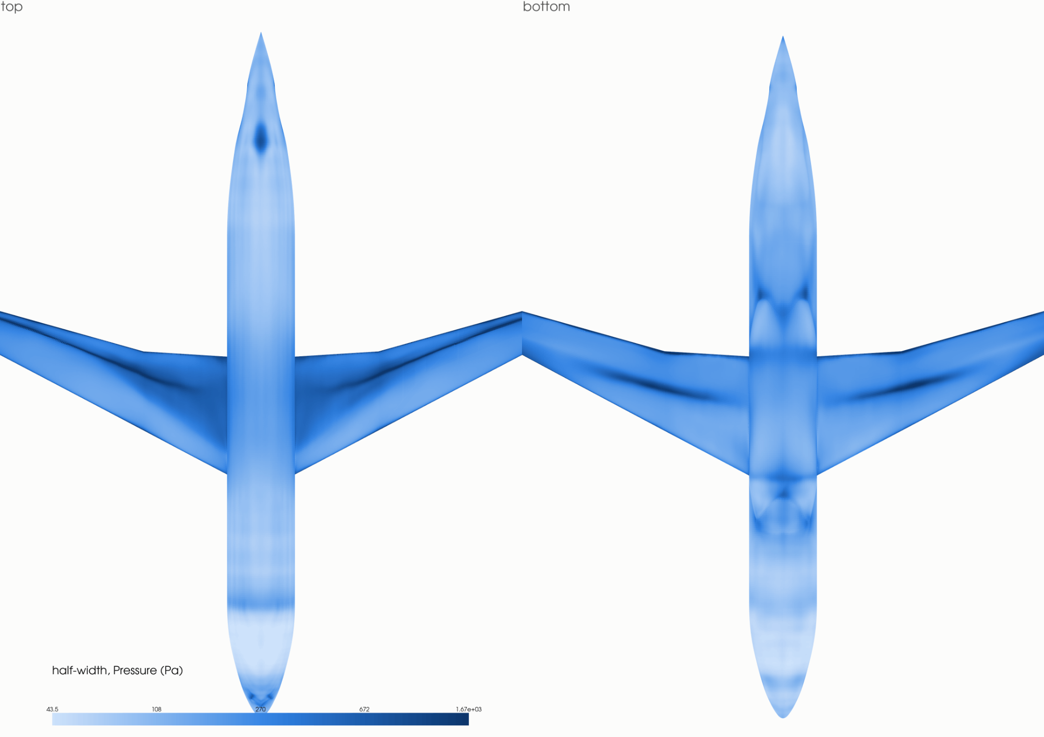
Figure 2. Calibrated pressure error-bar half-width (Pa) on the upper (left) and lower (right) surfaces of a held-out SHIFT-Wing design. The widest error bars form a spanwise band on the upper wing that follows the shock, and run along the leading edges.

The drag error bar is ±0.0014 in C_D, or 14 drag counts, on designs that span 135 to 1,080 counts. The lift error bar is ±0.009 in C_L. On 73 test designs, the CFD drag falls inside its error bar 69 times and the CFD lift 62 times. For 90% coverage on 73 designs, counts between about 61 and 71 are consistent with the target. Averaged over 500 random reshuffles of which designs calibrate and which test, drag and lift coverage both come to 91%.

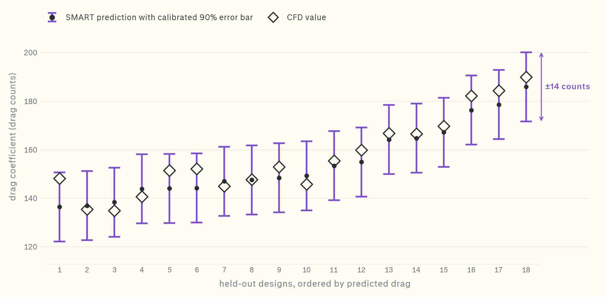
Figure 3. Predicted drag with calibrated 90% error bars (±14 counts) and CFD drag for 18 held-out SHIFT-Wing designs, ordered by predicted drag.

Figure 3 shows the 18 test designs whose predicted drag lies closest together, which is the situation a screening study faces. Designs 1 and 18 are clearly separated. Neighboring designs whose error bars overlap are tied within the model’s accuracy, and a screening study would send those to CFD.

SHIFT-SUV: coverage and drag

SHIFT-SUV is trained on about 2,000 full-scale AeroSUV variants, roughly half with estate rear ends and half with fastback rear ends. Each design has a 5.1-million-face surface mesh.

On 74 held-out designs, the calibrated error bars contain the CFD value at 90.0% of surface points. The widest error bars sit where the flow turns sharply: the A-pillars and mirrors, the front corners, the wheel arches, and the roof and rear edges. The narrowest are on the smooth door panels.

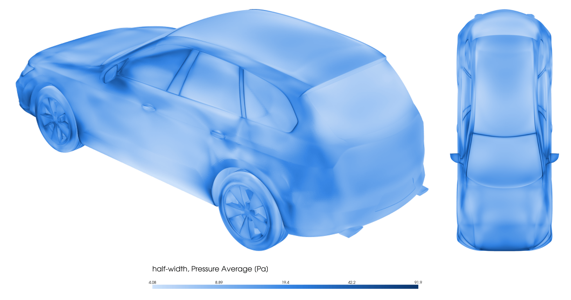
Figure 4. Calibrated pressure error-bar half-width (Pa) on a held-out SHIFT-SUV design, isometric and top views.

The drag error bar is ±0.0055 in C_d, or ±1.8% of drag. On 22 held-out designs evaluated on the full mesh, 19 fall inside their error bar, which is in line with 90% for a sample that size. The error bar is a tenth of the 0.055 spread in C_d across those designs.

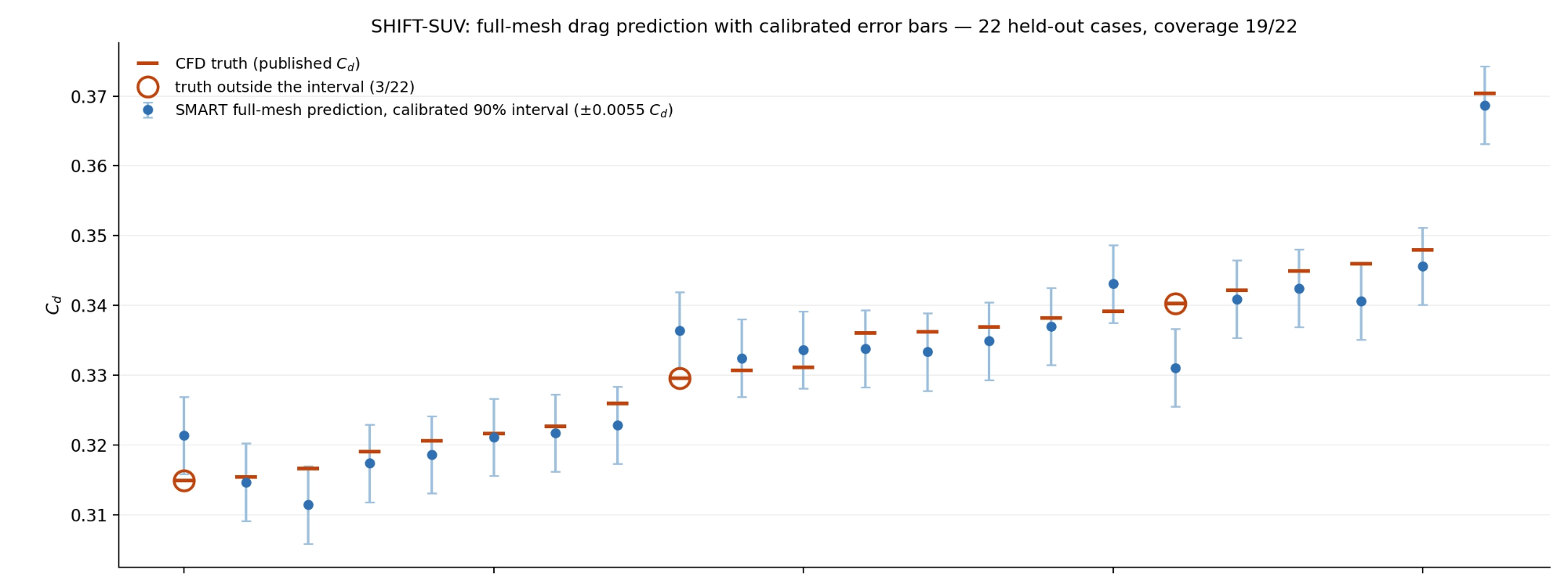
Figure 5. Full-mesh drag prediction with calibrated 90% error bars (±0.0055 in C_d) and CFD drag for 22 held-out SHIFT-SUV designs, ordered by CFD drag. 19 of 22 CFD values fall inside.

SHIFT-Truck: open-bed pickup

On SHIFT-Truck, the calibrated pressure error bar runs from about 13 Pa to about 230 Pa. The widest error bars are at the grille and front fascia, where the flow stagnates. The hood leading edge and the windshield base and header also carry wide error bars, which matches separation and reattachment there. The A-pillars and mirrors, the door and window seams, and the wheels and wheel arches follow. The narrowest error bars are on the door panels, the lower flanks and the roof center, where the flow stays attached. In the open bed, the rails and the cab back wall carry wider error bars than the bed floor, which is consistent with the recirculating flow behind the cab.

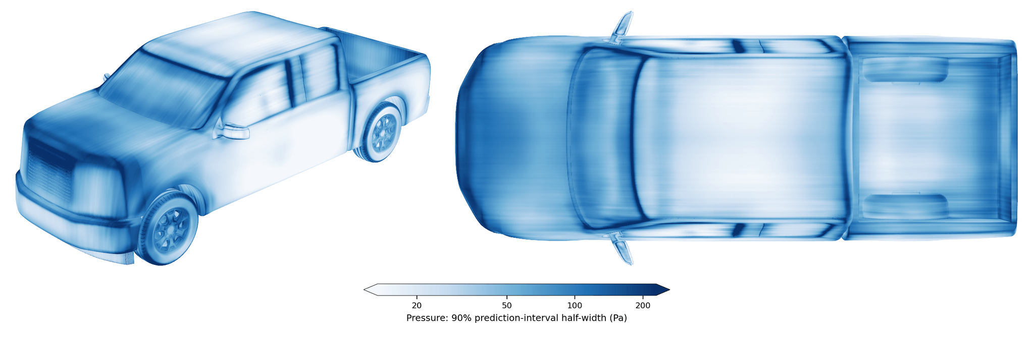
Figure 6. Calibrated pressure error-bar half-width on a held-out SHIFT-Truck design, isometric and top views, on a log scale.

The drag error bar is ±0.0088 in C_d, or ±2.2% of drag. On 49 held-out designs, 47 fall inside their error bar (Figure 7).

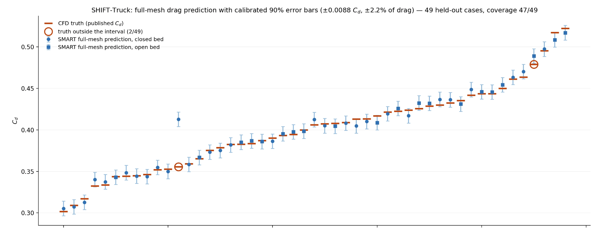
Figure 7. Full-mesh drag prediction with calibrated 90% error bars (±0.0088 in C_d) and CFD drag for 49 held-out SHIFT-Truck designs, closed bed (circles) and open bed (squares), ordered by CFD drag. 47 of 49 CFD values fall inside.

DrivAerML

DrivAerML is a public dataset of high-fidelity simulations of DrivAer car variants. The error bars concentrate at the grille, the hood leading edge, the windshield header and A-pillars, the mirrors, the wheels and wheel arches, the underbody and the rear diffuser. They stay low on the doors, the roof and the flat floor. On each car, the widest error bar is about 12 times the narrowest. The widths vary in the way the flow physics predicts: they are wide where an LPM is expected to struggle, such as the hood and the wheels, and narrow on smooth surfaces such as the roof.

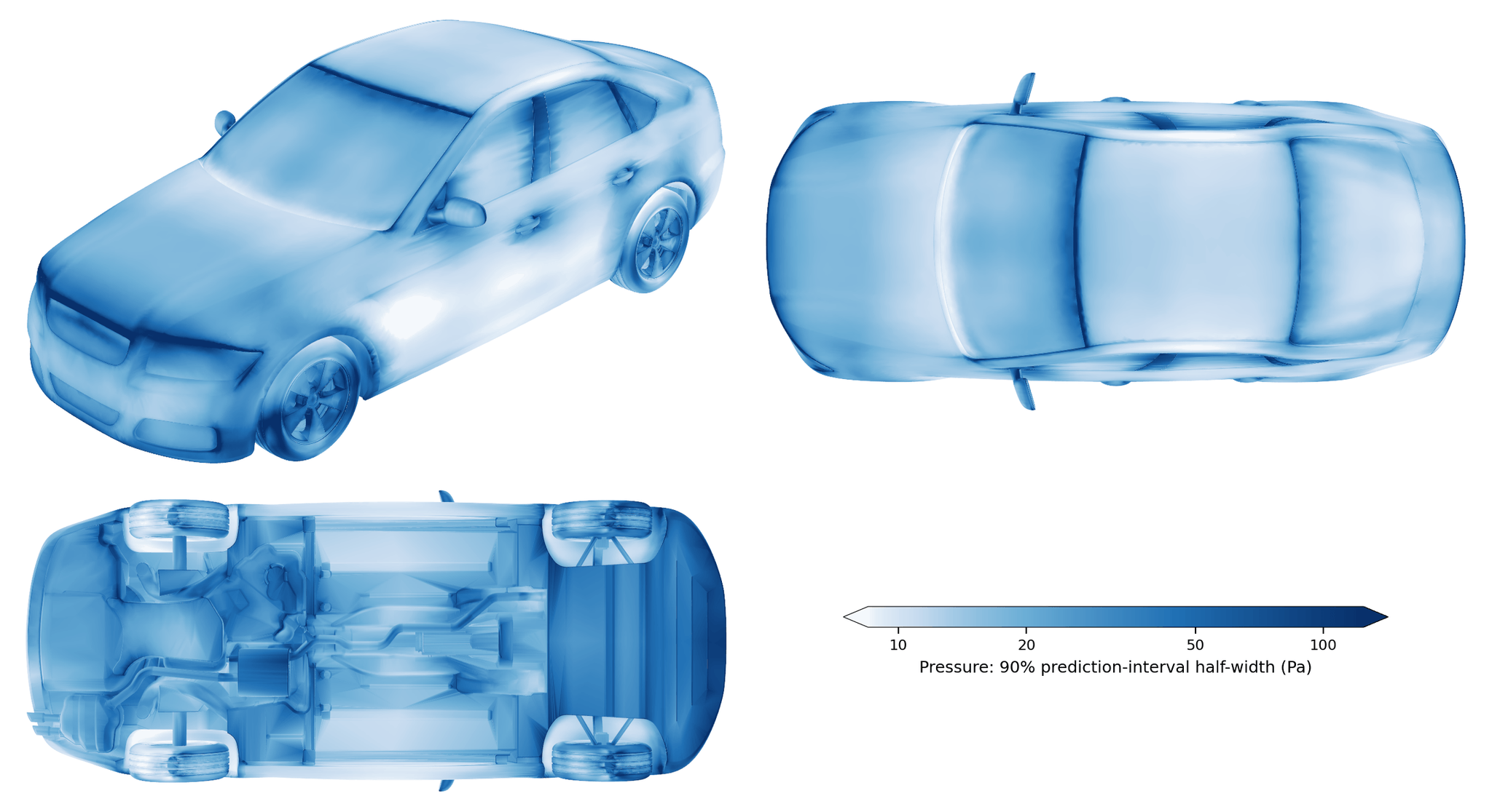
Figure 8. Calibrated pressure error-bar half-width on a held-out DrivAerML car, isometric, top and underbody views, on a log scale.

The drag error bars on DrivAerML vary from design to design, with a median of ±0.0097 in C_d, between 2.6% and 4.7% of drag. On 50 held-out designs, 44 fall inside their error bar (Figure 9).

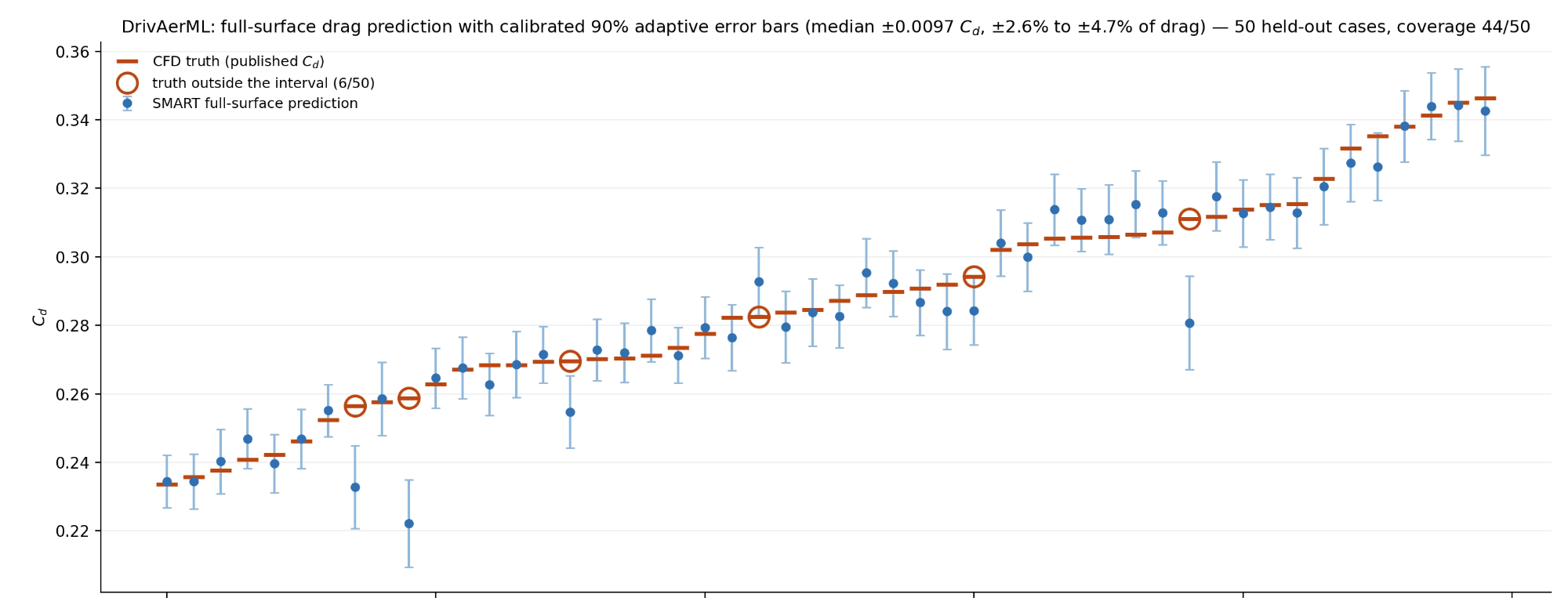
Figure 9. Full-surface drag prediction with calibrated 90% error bars and CFD drag for 50 held-out DrivAerML designs, ordered by CFD drag. 44 of 50 CFD values fall inside.

OOD detection and UQ together

The two methods cover different cases, and together they give a complete picture of trust in a Large Physics Model. The OOD score is computed first, before the LPM’s prediction. A design that falls outside the training distribution is flagged and sent to CFD, since UQ calibration holds only for designs that resemble the calibration set. For an in-distribution design, UQ sizes the answer at every surface point and for drag and lift. Across a study, the designs with the widest error bars show where the next CFD runs add the most to the training and calibration sets.

To see how Luminary builds model confidence into Large Physics Models, and what it can do for your design workflows, get in touch with our team or request a demo.

References

[1] M. C. Kennedy and A. O’Hagan, “Predicting the output from a complex computer code when fast approximations are available,” Biometrika 87(1):1–13, 2000. doi:10.1093/biomet/87.1.1

[2] H. Papadopoulos, A. Gammerman and V. Vovk, “Normalized nonconformity measures for regression conformal prediction,” Proc. 26th IASTED Int. Conf. on Artificial Intelligence and Applications (AIA 2008), pp. 64–69, 2008.

[3] J. Lei, M. G’Sell, A. Rinaldo, R. J. Tibshirani and L. Wasserman, “Distribution-free predictive inference for regression,” JASA 113(523):1094–1111, 2018. arXiv:1604.04173