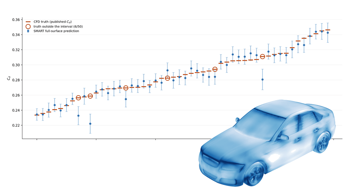
Six weeks before design freeze, the wing changes. The aerodynamic database, the table that guidance and controls, structural loads, flight simulation, and trajectory analysis all depend on, no longer describes the airplane. Rebuilding it means another simulation campaign while downstream teams wait for current forces and moments.
The new compute request carries an assumption: this will be the last geometry change of the program. Nobody expects that assumption to hold. The team is being asked to repeat much of the same simulation and validation work, knowing that the resulting database will stop describing the aircraft when the next change lands.
The aerodynamic database should be a capability the program maintains, not a deliverable it rebuilds.
That is achievable now. The reason has less to do with making an individual CFD solve faster than with changing what a simulation campaign leaves behind. Instead of producing a static table for one configuration, a sampled set of high-fidelity simulations can train a Large Physics Model that the program updates and reuses. The database becomes one output of that model rather than the final destination of the simulation effort.
How engineers keep case counts manageable
An aerodynamic database looks like a spreadsheet and gets budgeted like a test campaign.
For a given aircraft configuration, it maps flight conditions, including Mach number, angle of attack, sideslip, and control surface deflection, to the forces and moments on the vehicle and its control surfaces. Every row is one converged high-fidelity simulation at one condition. On a typical aircraft mesh, each case can cost hundreds of core-hours.
Seven control surfaces sampled at five settings each produce 5⁷, or roughly 78,000 control configurations, before the flight-condition grid gets layered on top. Guidance and controls derivatives multiply the total further because they require evaluations at perturbed conditions.
High-fidelity simulations remain essential because their assumptions and conditions are explicit and interrogable. Physics AI changes how that evidence is generated and reused; it does not eliminate it.
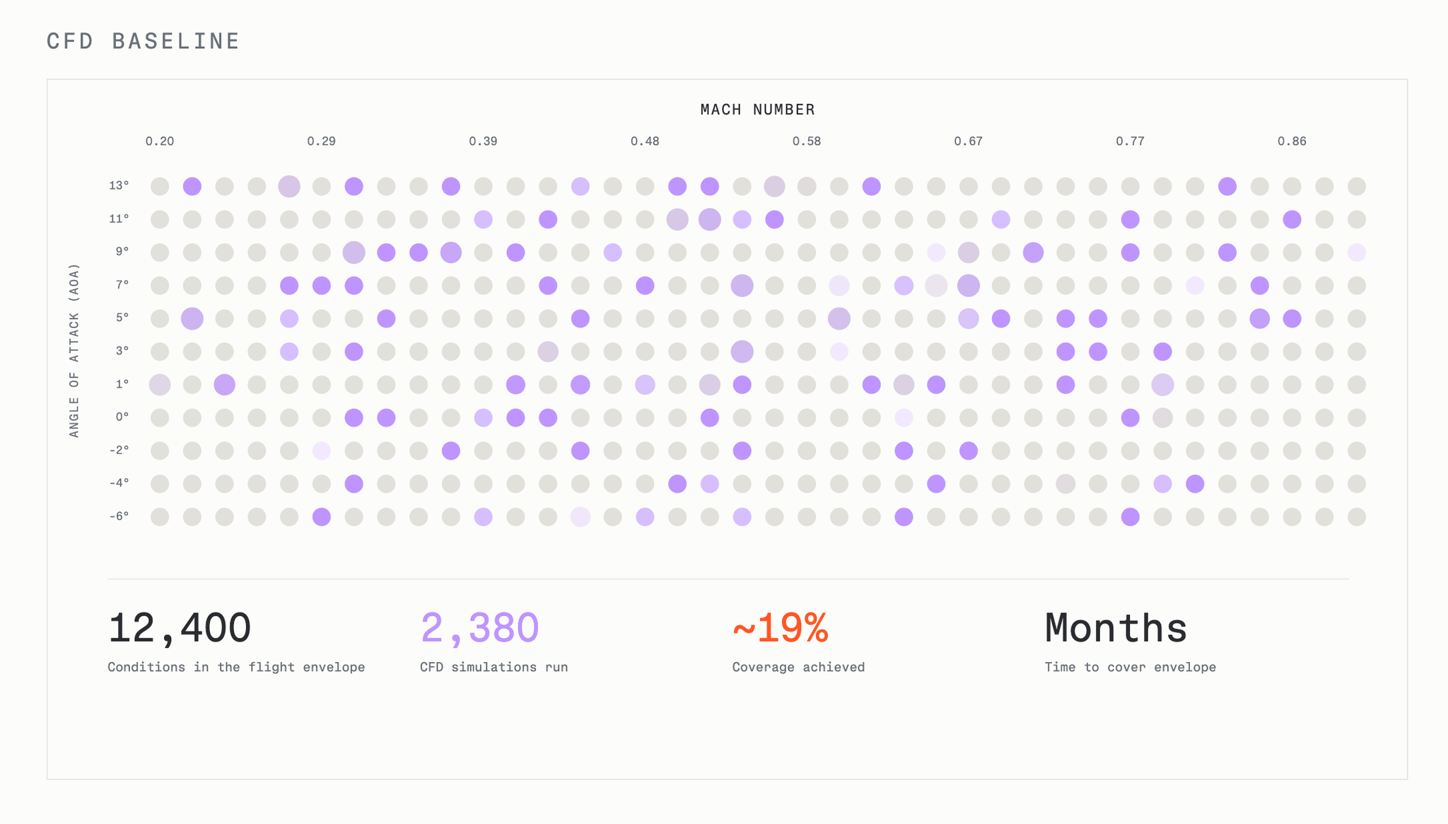
What is rarely attainable is complete coverage. A flight envelope sampled in Mach number and angle of attack alone can hold 12,400 conditions, and a campaign of 2,380 solves, running for months, populates about 19 percent of them. Teams generally keep the case count manageable in three ways, and each gives up something different.
- Semi-empirical tools such as panel codes give up reuse: a cheap low-order solve, corrected by hand against CFD, with corrections that must be retuned from scratch for every new geometry.
- Wind tunnel campaigns give up coverage: real physical measurement, but at a small number of points tied to the one configuration tested, on a schedule the design may outrun.
- Build-up sweeps give up fidelity: run each control surface separately and sum the results, 35 runs instead of thousands, which assumes the control surfaces do not interact. They interact. And the gaps between sampled conditions get filled by interpolation, which can put an abrupt change into a table a control loop was tuned against.
None of these methods tells an engineer how much to trust a condition that was never evaluated. The usual response to that uncertainty is to run more cases. The campaign stays expensive, remains on the critical path, and begins to depreciate as soon as the design or requirements change.
A Large Physics Model changes the resulting database across the dimensions that matter downstream:
| Dimension | Conventional aerodynamic database | Physics AI aerodynamic database |
|---|---|---|
| Coverage | Uses a sparse grid or additive control-surface sweeps | Populates combined configurations across the operating envelope |
| Fidelity | Relies on interpolation and may omit nonlinear interactions | Captures nonlinear interactions and predicts full aerodynamic fields |
| Confidence | Uses additional cases as a proxy for confidence | Identifies out-of-distribution queries and attaches uncertainty to predictions |
| Maintainability | Requires a new campaign when the geometry changes | Updates the trained model with targeted simulations |
| Reuse | Produces a static table for a specific configuration and application | Creates a reusable model that can support the database and downstream analyses |
Choose what to simulate, not what to omit
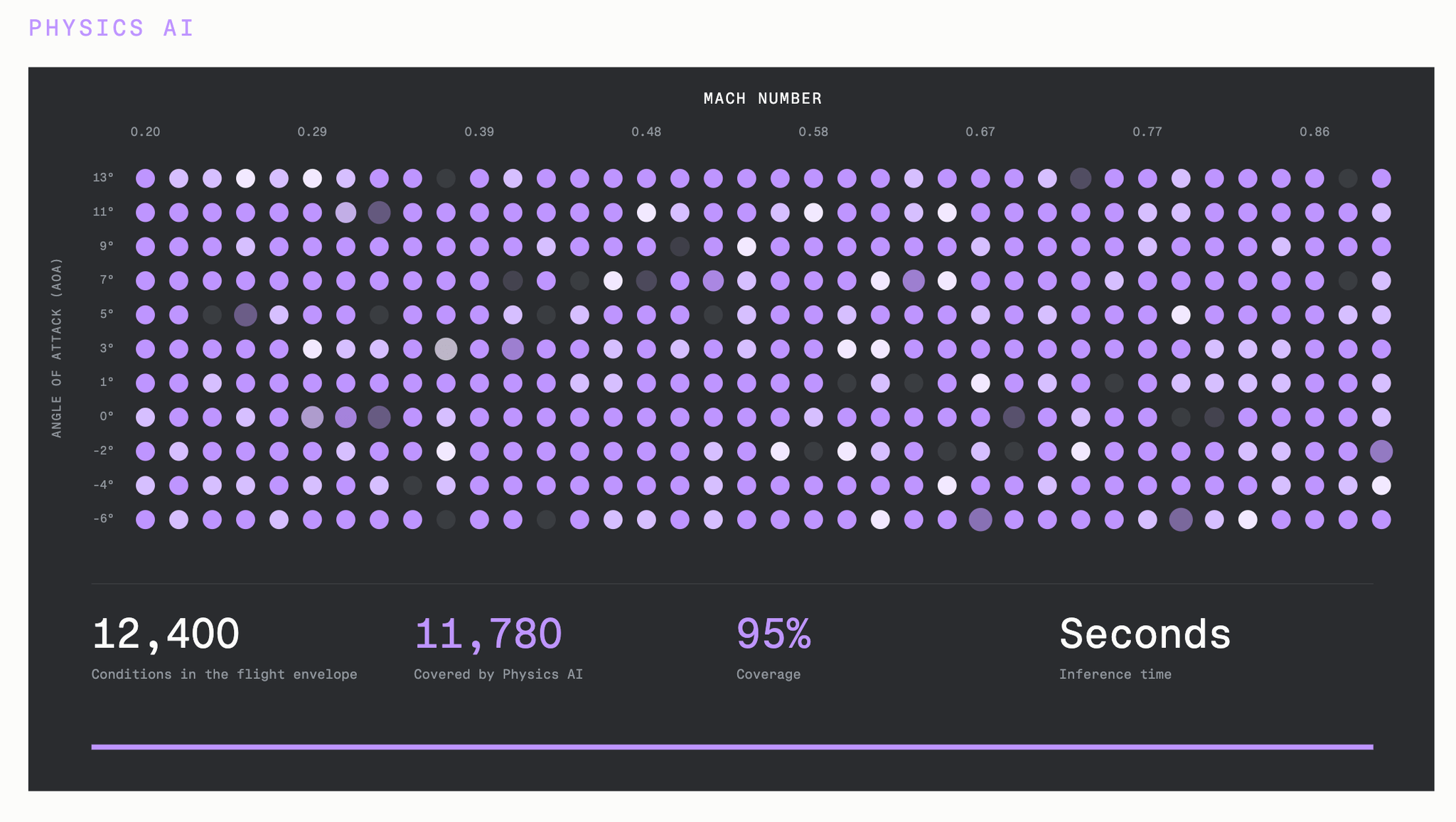
A Large Physics Model creates another option. Instead of deciding which interactions or portions of the operating envelope to omit, engineers choose a representative fraction of the design space to simulate and use those results to train a model that populates the rest.
Latin Hypercube Sampling distributes training points across the design space without requiring a dense grid. Engineers run high-fidelity simulations at those points and, when available, add wind tunnel measurements and operational telemetry. The same 2,380 solves that populate 19 percent of that envelope as a static table can instead train a model that predicts 11,780 of the 12,400 conditions, about 95 percent, in seconds each.
The trained model predicts aerodynamic fields at the operating conditions between the sampled points. Inference returns a result in seconds rather than the hours required for a CFD solve. It predicts pressure and wall shear across the geometry, not just a single lift or drag coefficient. The same prediction can populate the aerodynamic database and support structural loads analysis.
This does not remove CFD from the program. It changes how often engineers run it and what each run leaves behind. A simulation is no longer only one row in a table. It becomes training evidence for a model whose trusted operating envelope can expand over time.
That distinction changes the unit of work. Instead of completing a new table for each configuration, the program maintains a representation of the physics that carries forward to future database updates.
Speed and coverage alone, however, do not make the sampled approach defensible. Engineers also need to know whether a query is supported by the training data and how much uncertainty remains in the prediction.
Know when the model needs more evidence
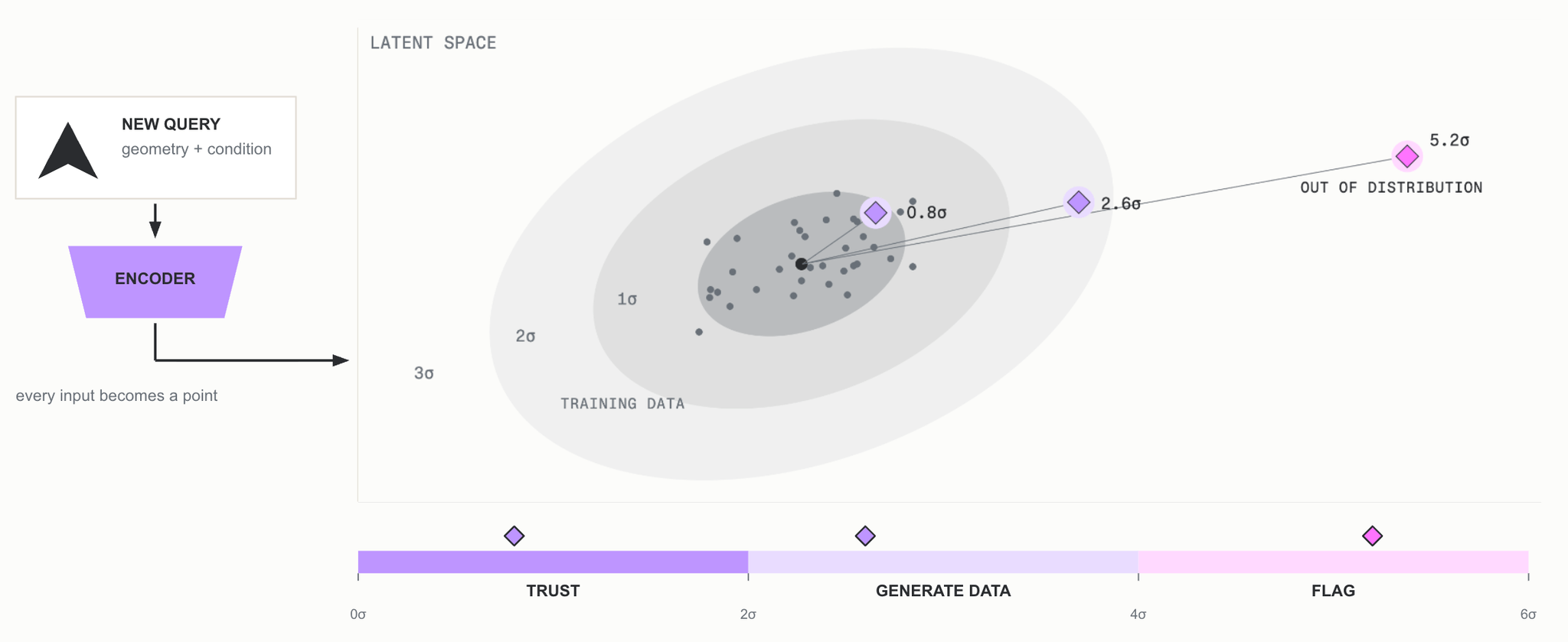
Out-of-distribution detection and uncertainty quantification provide complementary signals. The first asks whether a query is supported by the training data. The second estimates how much uncertainty remains in the resulting prediction.
During inference, out-of-distribution detection measures how far a query lies from the training distribution and therefore how far the model must extrapolate.
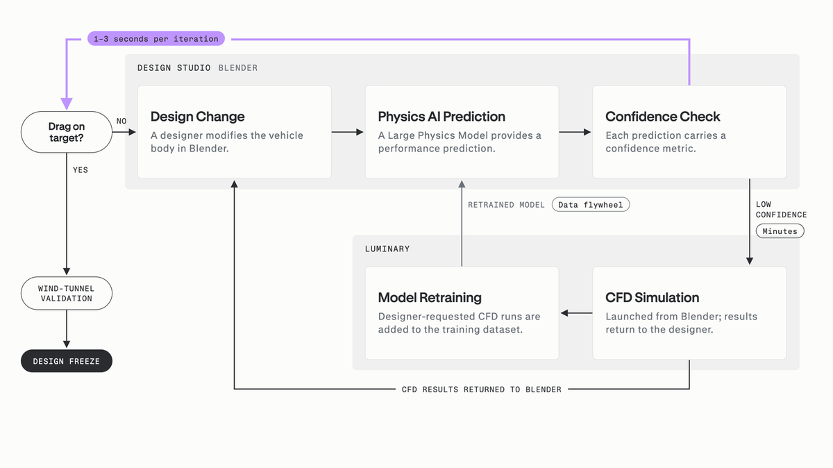
That distance sets the response. Queries close to the training distribution are answered as predicted. Queries at its edge are routed back to high-fidelity simulation, and each result is added to the training set. Queries far outside it are flagged rather than answered.
Even within that envelope, prediction error does not disappear. Uncertainty quantification attaches an error estimate to the result, so downstream teams can judge whether the prediction is ready for their analysis.
Together, these signals help engineers decide where the model has sufficient support and where another simulation or physical test is warranted. Instead of trying to cover every case in advance, the team adds evidence where the model indicates that it is needed. Each new solve expands the trusted envelope and strengthens a reusable capability.
The workflow does not replace engineering judgment. Engineers remain responsible for deciding when a prediction has sufficient support and when it requires confirmation through a full solve or physical test.
A geometry change becomes an update, not a restart
The value of a maintained model becomes clearest when the aircraft changes.
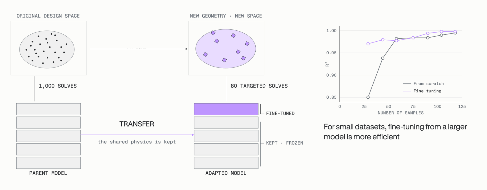
Through transfer learning, the model carries forward what it learned from the baseline configuration and updates that representation with data from the new geometry. Only the top layers are retrained; the rest keep the shared physics and stay frozen. A parent model built on 1,000 simulations can adapt to a new geometry on roughly 80 targeted solves, and at sample counts that small, fine-tuning from the parent reaches higher accuracy than training a fresh model from scratch.
Guidance and controls, loads, flight simulation, and trajectory teams can then work from an updated database built with targeted simulations. The model carries forward what the program has already learned, while its confidence mechanisms identify where the changed geometry requires new evidence.
One aerospace program has put this workflow into production. The team trained a Large Physics Model on several thousand simulations spanning Mach 0.1 to 8 and kept prediction error below 3 percent across that range. For each design iteration, the team now spends roughly $9,000 less on the simulation compute required to generate a new aerodynamic database.
The value extends beyond the original table. The team is applying the same trained pipeline to replace the CFD step in structural loads analysis, reusing the model and its confidence mechanisms in a second discipline.
From a recurring deliverable to a reusable asset
A faster CFD solver reduces the cost of an individual case. Physics AI changes what the campaign produces: instead of completing a fixed matrix that expires with the geometry, engineers maintain a continuously validated model that carries forward to the next configuration and the next downstream application.
That changes the question the program asks when the aircraft changes.
Today, the question is: “Can we afford to rebuild the aerodynamic database before the next design milestone?”
With a maintained model, it becomes: “Which conditions do we still need evidence for?”
That workflow is the subject of How One Aerospace Company Took Their Development from Discrete to Continuous with Physics AI.
For more on how Physics AI is changing the economics of engineering analysis, subscribe to the Physics AI newsletter.