“All models are wrong, but some are useful.” George E.P. Box wrote that decades before anyone trained a neural network on a CFD dataset, but every engineer who has shipped a simulation result into a design review has lived the second half of that sentence: useful only if you know how wrong.
Weather forecast models already do this: a rain forecast doesn’t just predict rain, it gives you a probability. Autonomous vehicle systems do the same, flagging when they’re uncertain about a pedestrian’s position or an unfamiliar scenario.
Yesterday: Trustworthy Physics Simulation
An aerodynamics engineer sizing a new wing used to have one tool: the solver. A CFD run took hours, sometimes longer, but the trust it earned was traceable. If the output looked wrong, the engineer knew where to look: mesh resolution, turbulence model assumptions, boundary condition simplifications, convergence tolerance. The outcome was reliable answers, purchased one design point at a time. A design cycle might afford a handful of configurations, because each one cost hours of compute and an engineer’s attention to verify.
Today: Fast Physics AI with Guardrails
Large Physics Models (LPMs) change that economics. Deep learning architectures such as Luminary-SMART, DoMINO and GeoTransolver, trained on high-fidelity simulation data, predict complex physical phenomena in seconds instead of hours. The same engineer can now sweep thousands of angles of attack, Mach numbers, and wing geometries in the time a single solver run used to take. That speed is the whole point of adopting Physics AI.
It’s also the problem. An LPM is still a neural network, and it inherits deep learning’s core vulnerability: presented with an input, a standard neural network returns a definitive answer, even when it’s blindly guessing. Unlike the solver, there’s no defined place to look when the answer is wrong. It just looks right, and nothing about the output tells the engineer which of those thousand results to trust. Trusting an LPM means getting an answer to two questions it doesn’t answer on its own: how sure am I about the question, and how sure am I about the prediction.
Out-of-Distribution Detection: How Sure Am I About the Question?
Out-of-Distribution (OOD) detection is the mechanism that lets a model recognize when an input falls outside the bounds of its training data.
The model can reasonably predict physics for a new geometry or flow condition, as long as that input falls within the bounds of its training data. For example, if a model is trained using various aircraft geometries and operating conditions and we query the same model on a car geometry, the model needs to recognize that the input sits far outside anything it has seen.
When a general computer vision model encounters an out-of-distribution input, the failure is obvious to a human: researchers have shown state-of-the-art image classifiers label pure generated noise as a cheetah with 99.9% confidence.
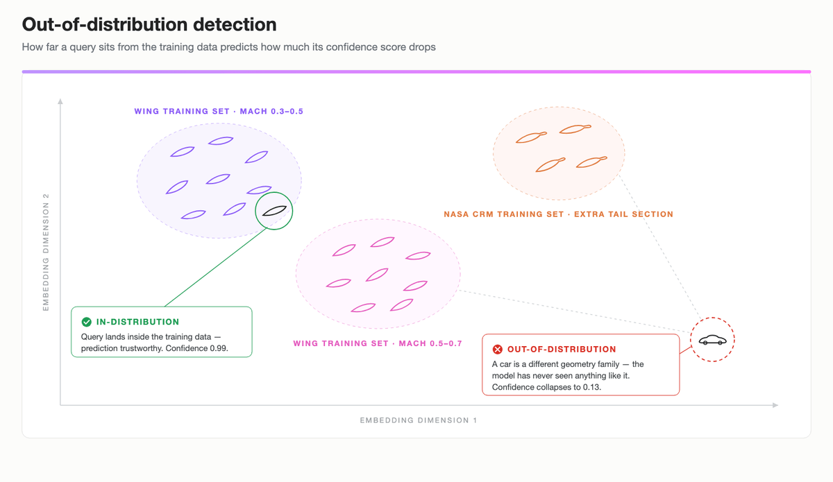
For an LPM, the same failure is harder to catch, because it requires a CFD expert to spend hours looking at the field outputs to evaluate the validity of the predictions. Further, when used in a design exploration study, the faster a design search runs, the more configurations it tries, and the more of those configurations end up pushed beyond the training distribution by a drastically higher Reynolds number, a laminar-to-turbulent transition, or an unseen geometry. Without OOD detection, the model can produce convincing fields instead of raising a flag.
Uncertainty Quantification: How Sure Am I About the Answer?
Uncertainty Quantification (UQ) is the mechanism that gives a prediction a margin of error instead of a single number.
OOD detection covers inputs the model has never seen. UQ covers a second, related gap in the same design search: the design stays technically within the training bounds, but lands in a region where training data was thin, so the prediction is inexact even though it looks just as confident as anywhere else in the space. Without a confidence signal, both cases get predicted with the same false certainty, and the engineer can end up pushing a design to manufacturing that fails in physical testing. That’s why the model needs to output “450 MPa ± 15 MPa” instead of “450 MPa,” with the margin of error meaning something rather than being decorative.
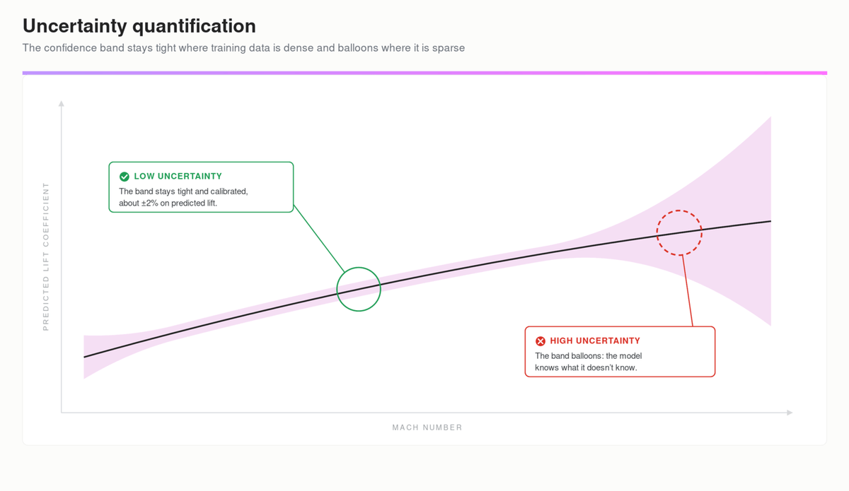
Together, OOD detection and UQ give an engineer both answers before trusting an LPM’s output. Getting that signal, today, runs into a compute problem, and it’s a problem in direct tension with the reason LPMs got adopted in the first place. The leading UQ methods were built for general deep learning, and scaling them to LPMs is expensive:
| Method | Training Cost | Inference Cost | Reliability Focus |
|---|---|---|---|
| MC Dropout | ~1X | ~50X | Aleatoric and epistemic |
| Deep Ensembles | ~5X | ~5X | Aleatoric and epistemic |
| Quantile NNs | ~2X | ~2X | Aleatoric only |
| Variational Inference (Bayesian Neural Networks) | ~3X | ~50X | Aleatoric and epistemic |
MC Dropout needs 50 or more forward passes per prediction, turning a 10-second inference into 10 minutes and erasing the speed advantage that justified moving to Physics AI. Deep Ensembles multiply training time and, worse, GPU memory: five copies of a model processing a large 3D point cloud can trigger out-of-memory errors even on high-end GPUs. Quantile networks are cheaper but only capture aleatoric uncertainty (noise in the data), not epistemic uncertainty (the model’s own lack of knowledge), so they can say “I’m not sure about my answer” but never “I don’t know this question,” which means they can’t do OOD detection at all. Bayesian neural networks are mathematically rigorous, notoriously unstable to train, and still need dozens of costly forward passes at inference.
The outcome, today, is a design search that’s fast in exactly the way that creates the risk: an engineering team gets to choose between sacrificing the speed advantage of the LPM, burning GPU budget nobody planned for, or skipping model confidence and flying blind. All three are already happening somewhere in a design review, whether or not anyone has named the problem yet.
How Luminary Builds Model Confidence
Luminary’s approach evaluates the input directly instead of running the LPM dozens of times to measure output variance. We project incoming geometry and parameters into a structured embedding space and use a lightweight metric to report the model’s confidence before the heavy physics inference even starts, so the overhead is negligible. The same design search that used to trade speed for trust now gets both.
We tested this (Luminary-OOD, on the SHIFT-Wing dataset, using the Luminary-SMART model) by establishing a baseline confidence score for strictly in-distribution inputs, then introducing increasingly severe distribution shifts:
| Test Case | Distribution Shift Type | Mean Confidence Score |
|---|---|---|
| Baseline (in-distribution) | Standard training distribution | 0.99 |
| Mild Mach shift | Slight deviation in Mach number | 0.92 |
| High Mach shift | Large deviation in Mach number | 0.82 |
| NASA CRM | Slight geometric shift (extra tail section); no change in other parameters | 0.57 |
| SUV geometry | Massive geometric shift; no change in other parameters | 0.13 |
The detector tracks an engineer’s intuition. A score of 0.92 reads as “slightly outside my comfort zone, proceed with caution.” Feed an aircraft aerodynamics model a bluff body like a car, and the score drops to 0.13, triggering a hard stop.
For that same wing design search, the outcome changes completely. The engineer can still sweep thousands of configurations at LPM speed, but every candidate now comes back with a confidence score attached. A design sitting at the edge of a sparse but valid region is worth a second look. A design the model is genuinely guessing on is worth a hard stop.
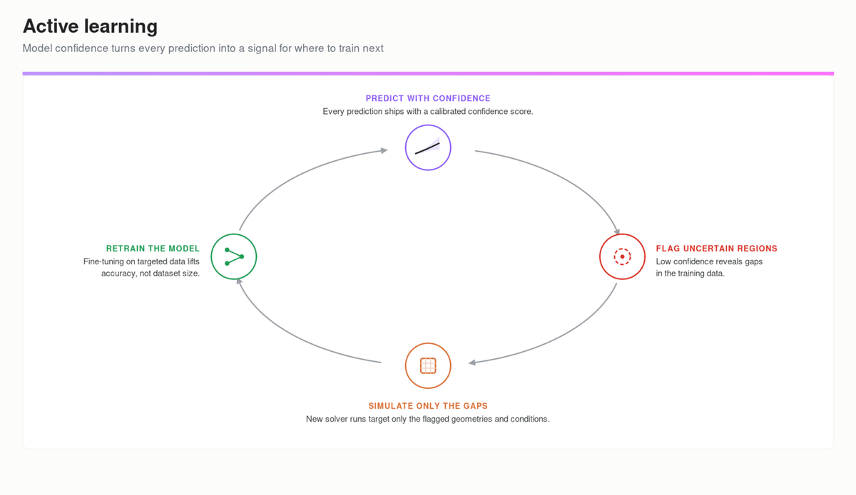
The same signal opens a second door: active learning. Because the model can point at exactly where it’s uncertain, teams can run new solver simulations only for the geometries and conditions the model doesn’t understand yet, instead of brute-force grid searches that spend compute re-confirming what the model already knows. That targeting can shrink a training dataset while holding accuracy steady, and it keeps working after deployment, flagging when a model needs retraining based on the operational data it sees in production. The same uncertainty estimate also feeds Bayesian optimization, letting the design search mathematically balance exploiting known good designs against exploring the uncertain regions that might contain the next breakthrough, this time with a way to tell the difference between the two.
Trustworthy Physics AI starts with a model that knows what it doesn’t know. To see how Luminary builds model confidence into Large Physics Models, and what it can do for your design workflows, get in touch with our team or request a demo.