Acoustic Point Sources: FW-H Against Direct CFD

Overview

An acoustic point source of a given multipole order (monopole, dipole or quadrupole) radiates a tone whose angular distribution depends on the order. This case places each source at the centre of a box, predicts the radiated sound with the Ffowcs Williams-Hawkings analogy evaluated on a permeable surface around the source, and compares it with the pressure the flow solver computes directly at the same observer points.

Problem Setup

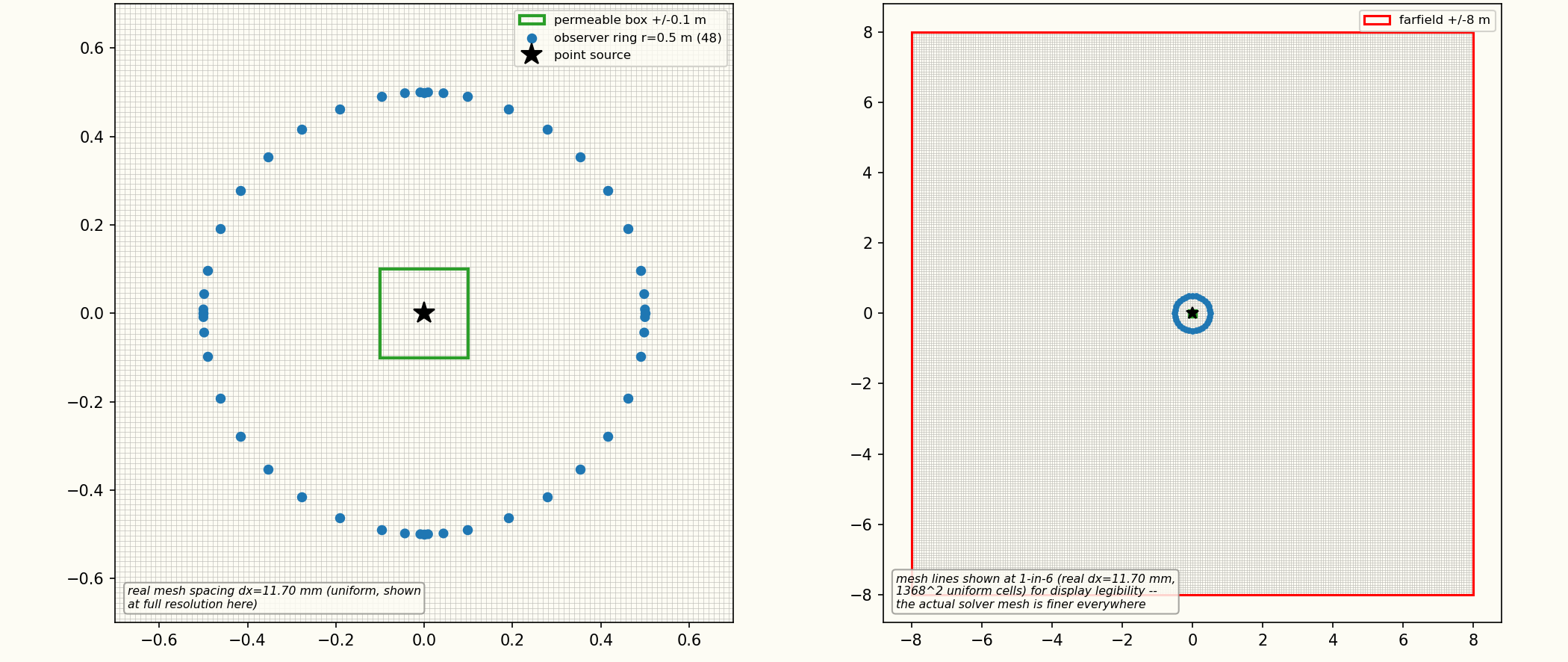
The flow is two-dimensional. The domain is a square of half-width $8$ m, represented by a slice $0.0125$ m thick with periodic faces, so the solution does not vary across it. It is filled with a still, laminar ideal gas at $p=101325$ Pa and $T=288.15$ K with a constant dynamic viscosity of ${10}^{-3}$ kg/(m s). The source is a Gaussian energy source of width $0.05$ m, driven at $2722$ Hz with a ramp over its first three periods, and the pole separation of the dipole and quadrupole is $0.02$ m. The Ffowcs Williams-Hawkings surface is a closed permeable box $0.2$ m on a side. The Ffowcs Williams-Hawkings integral is three-dimensional, so to give the sound of this two-dimensional source it is repeated over 400 copies of the slice along the span, which together act as a long line source. The observers are 48 points on a ring of radius $0.5$ m about the source, clustered near the $0^{\circ }$, ${90}^{\circ }$, ${180}^{\circ }$ and ${270}^{\circ }$ nulls of the multipole patterns. Time integration is second-order implicit with $\Delta t=1.84\times {10}^{-5}$ s and 1200 steps.

Quantities of Interest

The level of the source tone at each observer, from the Ffowcs Williams-Hawkings prediction and from the directly simulated pressure, over the interval before the first reflection from the domain boundary reaches the observer.

Discussion

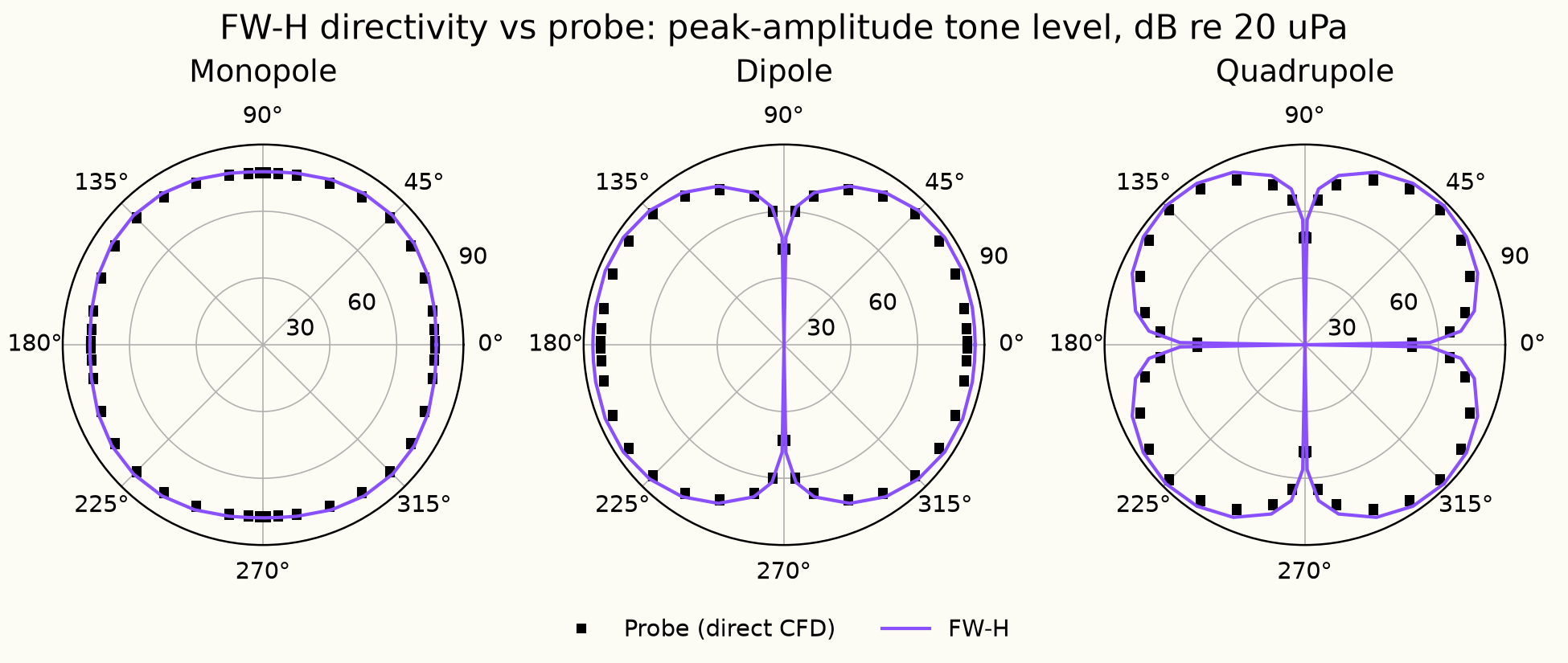
Each panel of the tone-level plot is a polar plot. The angle is the direction from the source, and the distance from the centre is how loud the tone is there, in decibels (dB). A monopole sends the same level in every direction, so its curve is a circle. A dipole is loud to the left and right and silent straight up and down. A quadrupole has four loud lobes with a silent direction between each pair. The Ffowcs Williams-Hawkings (FW-H) prediction reproduces each of these patterns, including the silent directions, and the pressure the solver computes at the observers follows the same shapes.

The two are not expected to match exactly. The FW-H method takes the flow solution on a small box around the source and carries the sound from there to each observer with a formula that is exact for sound travelling through still air, so nothing is lost on the way. The direct CFD (computational fluid dynamics) value is the wave after the solver itself has carried it across the grid to the observer, and every cell it passes through takes a little energy out of it. This numerical dissipation grows with the distance travelled and with how few cells each wavelength is spread over. The directly computed level therefore tends to sit slightly inside the FW-H curve, most visibly on the lobes of the quadrupole, and a difference of a few decibels between the two is expected.