
Manufactured Solution: Viscous (Navier–Stokes)
verification
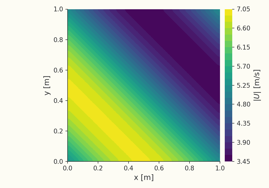
Overview
The Method of Manufactured Solutions checks that a discretization is implemented as intended and attains its theoretical order of accuracy. Rather than seeking a physically meaningful flow, one prescribes a smooth analytic field, inserts it into the governing equations, and analytically derives the source term required to make that field an exact solution. Running the solver with those sources yields a problem whose answer is known at every point, so the error can be measured directly and its convergence under grid refinement compared against the scheme's design order. This case exercises the compressible Navier–Stokes path, convection, viscous diffusion, and the energy equation together.
Problem Setup
The manufactured field is a smooth, fully three-dimensional sinusoid chosen so that every primitive variable has non-zero gradients in all directions and the flow stays subsonic and realizable. Writing , the primitive variables are
with density from the ideal-gas law . The amplitude is 3 and the wavenumber is ; the gas constant follows from the molecular weight. The source terms that make this field satisfy the equations are formed analytically and added to the residual; viscosity and thermal conductivity are constant. The domain is the unit cube, discretized by a family of uniform hexahedral grids at cells, each a 2× refinement of the last, so the global grid size halves at every level. Each grid is converged until the iterative residual is several orders below the discretization error, so the measured error is spatial.
Quantities of Interest
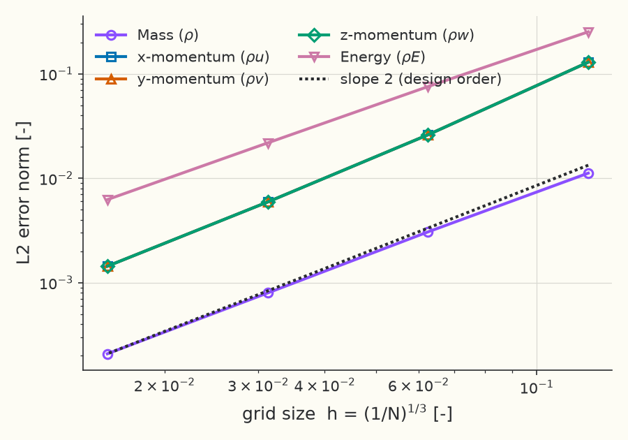
For each grid the solver reports the error of every conservative equation, mass, the three momentum components, and energy, as an norm over the domain. The verification examines two quantities: the decay of the error on a log–log plot of error against relative to the design slope of 2, and the observed order of accuracy, computed from the error ratio between successive grids. Across the four grids the momentum equations give observed orders of 2.310, 2.138, and 2.043, approaching 2 from above; the mass equation gives 1.870, 1.942, and 1.935; and the energy equation gives 1.743, 1.791, and 1.804. On the finest pair of grids the observed order is for momentum, for mass, and for energy.
Results
Discretization error vs grid size
Observed order of accuracy
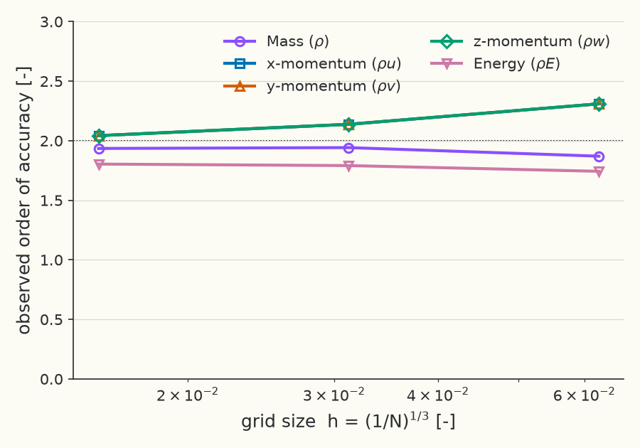
Observed order of accuracy per equation
| Equation | 512→4096 | 4096→32768 | 32768→262144 |
|---|---|---|---|
| Mass () | 1.870 | 1.942 | 1.935 |
| x-momentum () | 2.310 | 2.138 | 2.043 |
| y-momentum () | 2.310 | 2.138 | 2.043 |
| z-momentum () | 2.310 | 2.138 | 2.043 |
| Energy () | 1.743 | 1.791 | 1.804 |
Solver configuration
- features exercised
- Verification3DLaminarIdeal gasSteadyEnergy equation