
Manufactured Solution: Inviscid (Euler)
verification
Overview
The Method of Manufactured Solutions verifies that a discretization is implemented correctly and attains its design order of accuracy. A smooth analytic field is prescribed and substituted into the governing equations, and the source term that makes the field an exact solution is derived analytically. The solver is then run with those sources, so the solution is known everywhere and the discretization error can be measured exactly. Here the manufactured field is forced through the inviscid Euler equations: with viscous diffusion switched off, the case exercises the convective discretization and the gradient reconstruction.
Problem Setup
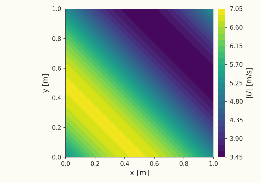
The manufactured field matches the viscous companion case: a smooth three-dimensional sinusoid with non-zero gradients of every primitive variable in all directions, kept subsonic. With ,
and density from the ideal-gas law . The analytic Euler source terms for this field are added to the residual. The domain is the unit cube on a family of uniform hexahedral grids at cells (uniform 2× refinement, so the grid size halves each level). The discretization uses no limiter, and each grid is converged until the iterative residual is below the discretization error.
Quantities of Interest
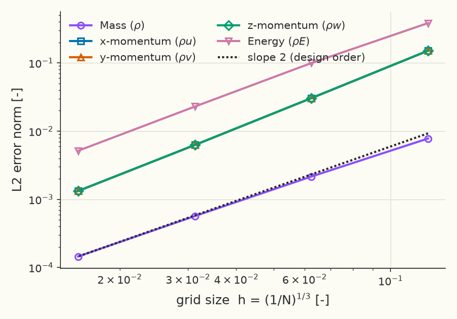
For each grid the solver reports the error of every conservative equation, mass, the three momentum components, and energy. The error is plotted against on a log–log axis alongside the design slope of 2, and the observed order of accuracy is computed from successive-grid error ratios. Across the three grid pairs the observed order is 1.85–1.97 for mass, 2.24–2.31 for each momentum component, and 1.95–2.15 for energy.
Results
Discretization error vs grid size
Observed order of accuracy
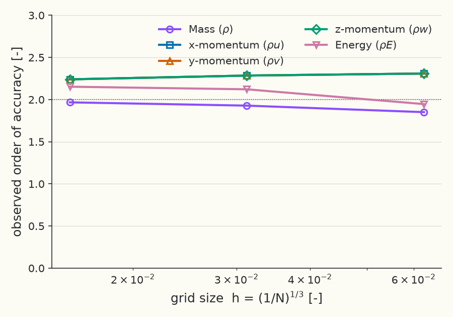
Observed order of accuracy per equation
| Equation | 512→4096 | 4096→32768 | 32768→262144 |
|---|---|---|---|
| Mass () | 1.851 | 1.928 | 1.967 |
| x-momentum () | 2.309 | 2.285 | 2.240 |
| y-momentum () | 2.309 | 2.285 | 2.240 |
| z-momentum () | 2.309 | 2.285 | 2.240 |
| Energy () | 1.947 | 2.122 | 2.153 |
Solver configuration
- features exercised
- Verification3DInviscidIdeal gasSteadyEnergy equation