LAGOON Landing Gear: FW-H Against Literature

validation

Validation 3D DES/LES Ideal gas Unsteady Energy equation FW-H (solid / permeable surface)

(a)

(b)

Animations of (a) isosurfaces of the Q-criterion around the gear, coloured by the velocity magnitude in m/s, and (b) the divergence of the velocity (the dilatation) on a plane through the gear. The turbulent wake appears as strong small-scale fluctuations in the dilatation.

Overview

The LAGOON landing gear is a simplified two-wheel main gear with a support leg, measured in a wind tunnel for the validation of flow and noise prediction methods. This case simulates the flow with a wall-modelled large-eddy simulation (WMLES) and predicts the far-field sound with the Ffowcs Williams-Hawkings analogy, evaluated on the gear wall and on a permeable surface around the gear in the same flow solution. The far-field spectra, the wall-pressure spectra at the kulite taps, the pressure coefficient around the wheel and the wake velocity statistics are compared with the measurements of Manoha et al. (2008, 2009).

Problem Setup

The flow is at $M_{\infty} = 0.23$ ( $U_{\infty} = 78.99$ m/s, $T_{\infty} = 293.56$ K, $p_{\infty} = 99448$ Pa). The turbulence is resolved with a large-eddy simulation using the Vreman subgrid-scale model and a wall model on the gear surface, with the FDS convective flux and its hybrid low-dissipation formulation, and second-order implicit time integration with $Δ t = 1.9 \times 10^{- 5}$ s. A sponge layer that absorbs the outgoing sound starts 3 m from the origin and is 2 m thick.

The flow is first advanced 20,000 time steps from freestream values to let the start-up transient pass, then 21,000 more, over which the acoustic and probe records are collected. The acoustic pressure is recorded 6 m from the origin at $60^{\circ}$ , $90^{\circ}$ and $120^{\circ}$ , both in the flyover plane $y = 0$ and on the sideline. The permeable surface is the box $- 0.16 \leq x \leq 0.25$ , $- 0.2 \leq y \leq 0.2$ , $- 0.3 \leq z \leq 1.18$ m. Probes record the pressure at the kulite taps and on a ring around the wheel, and the velocity along the wake lines.

Quantities of Interest

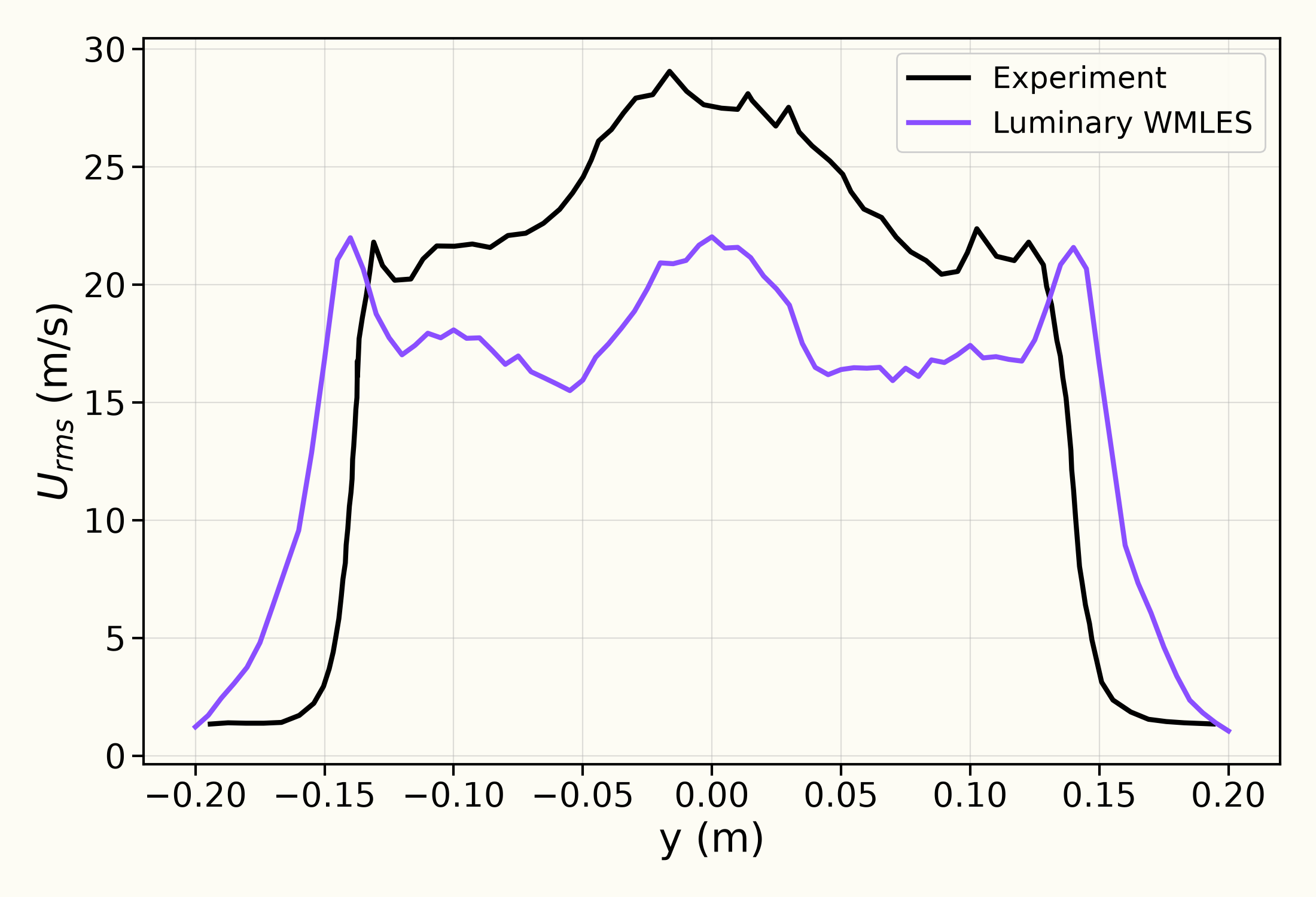
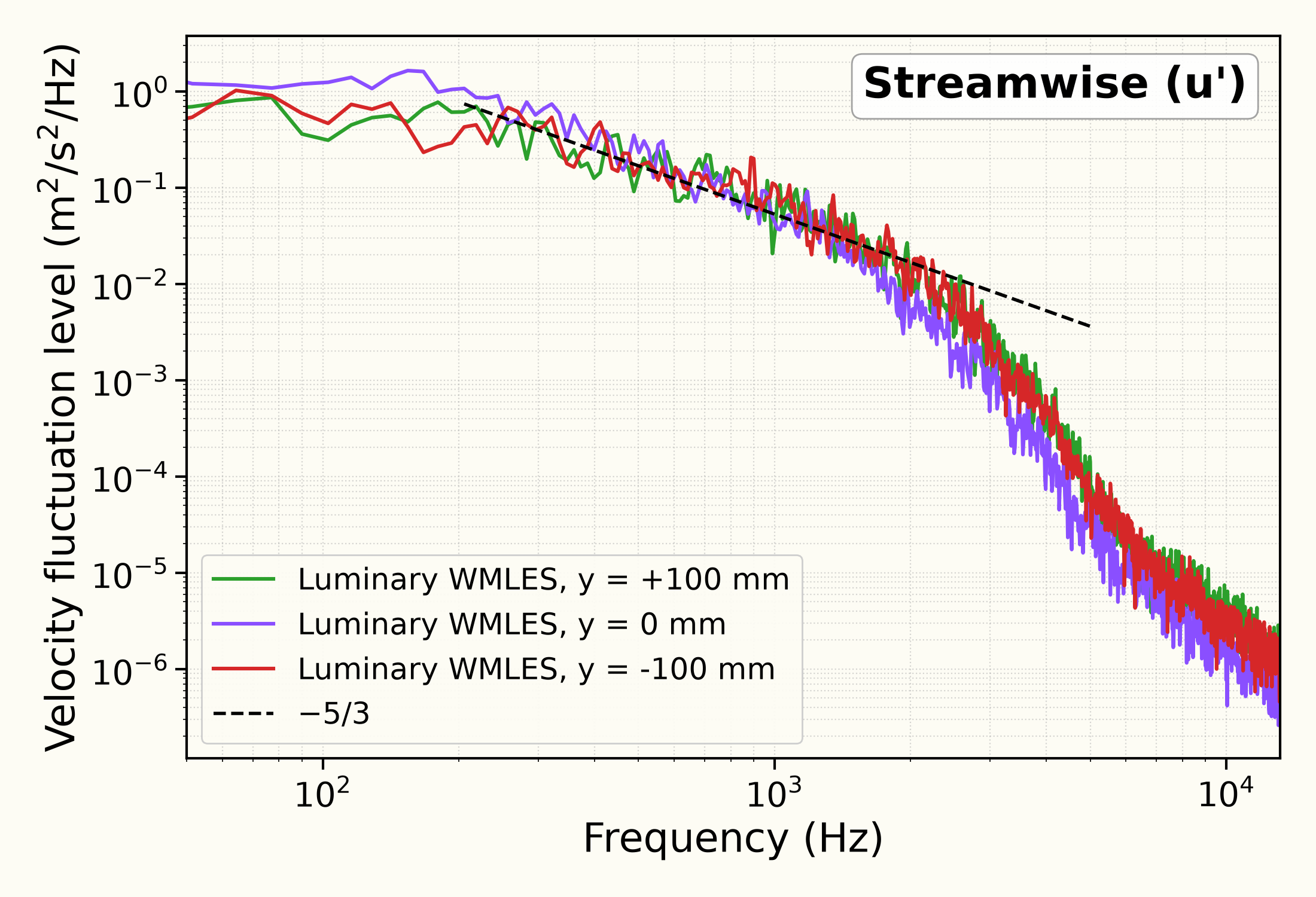
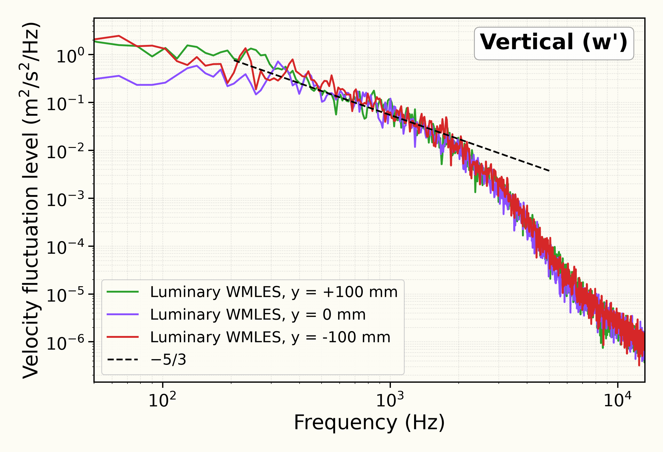
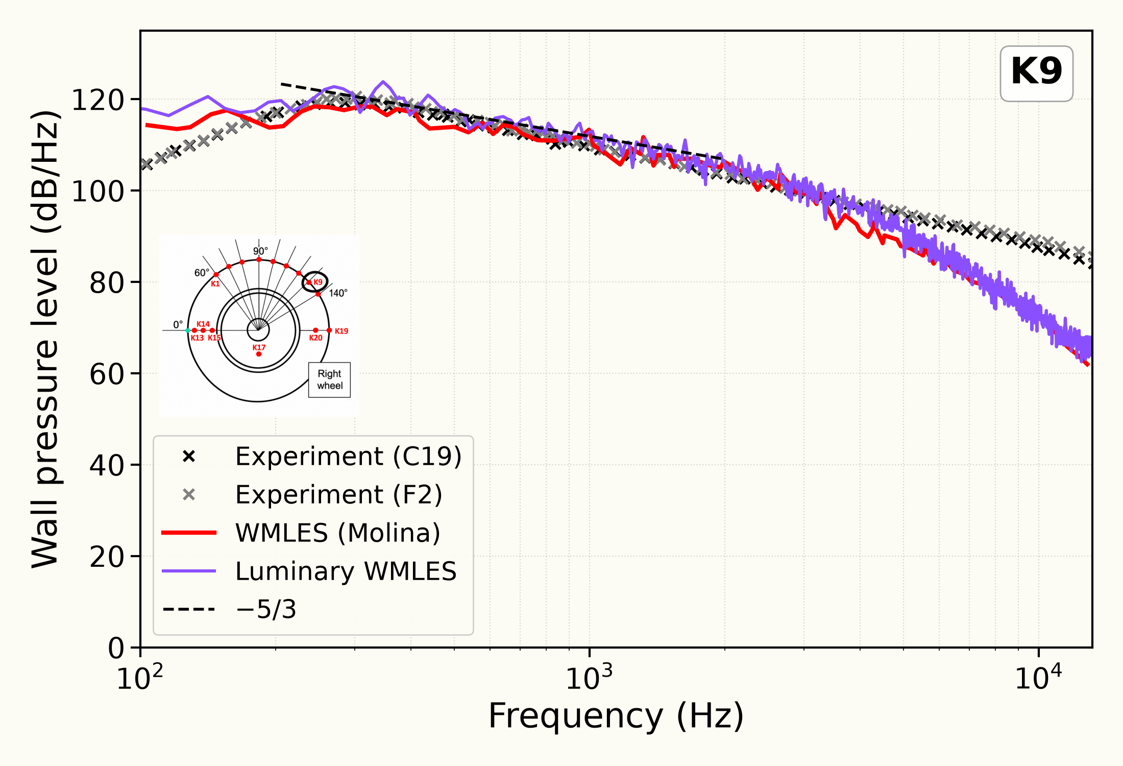
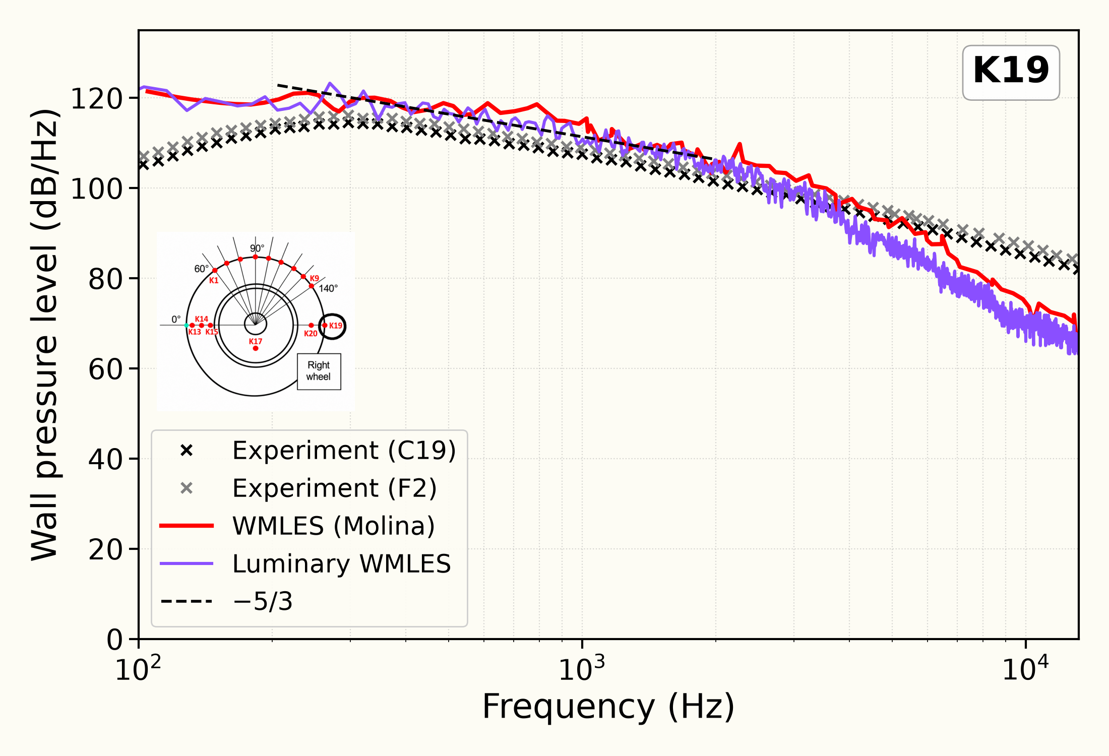
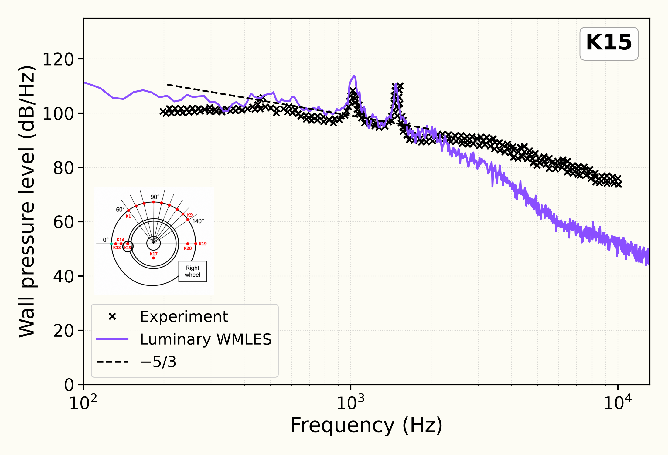
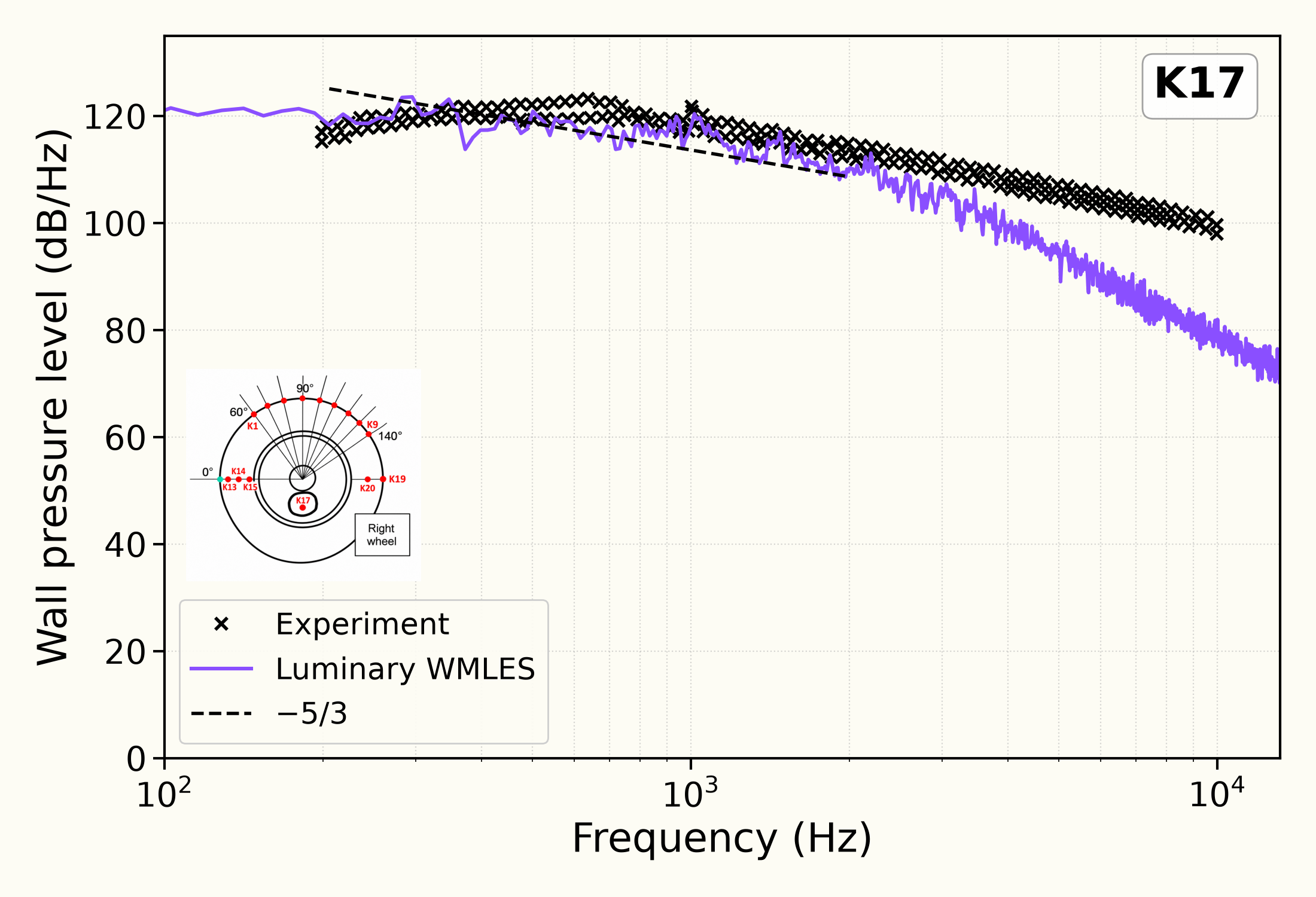
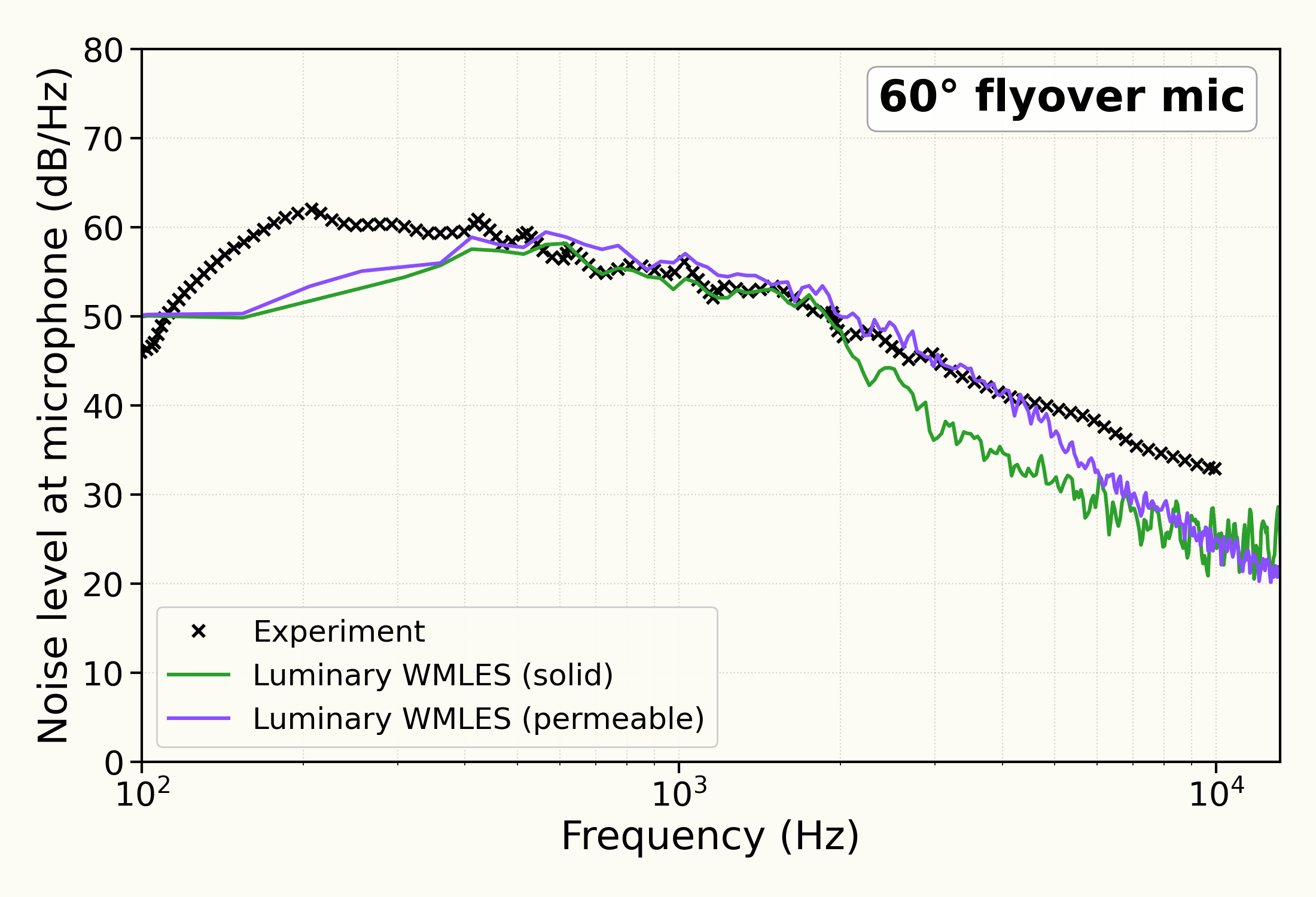
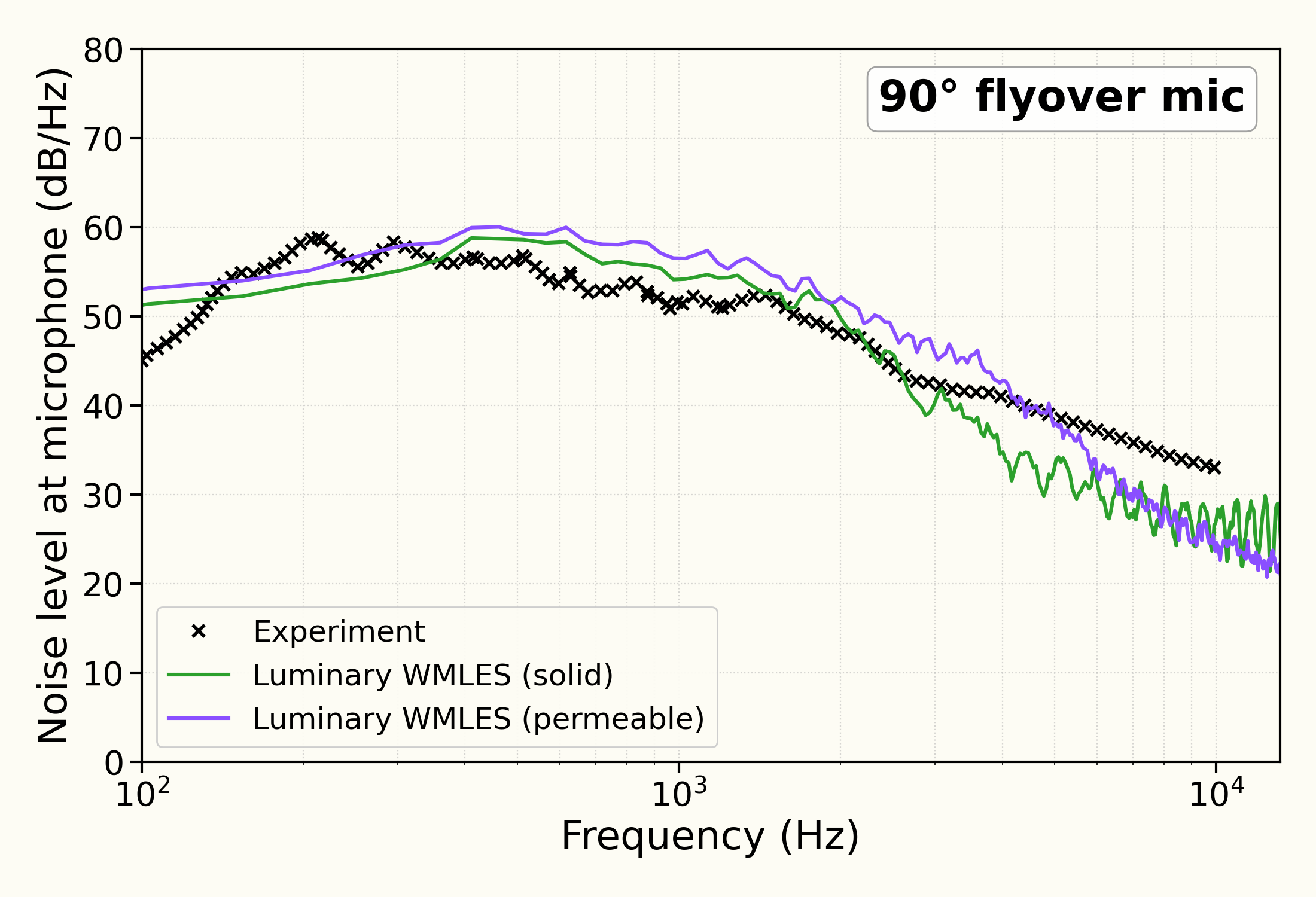
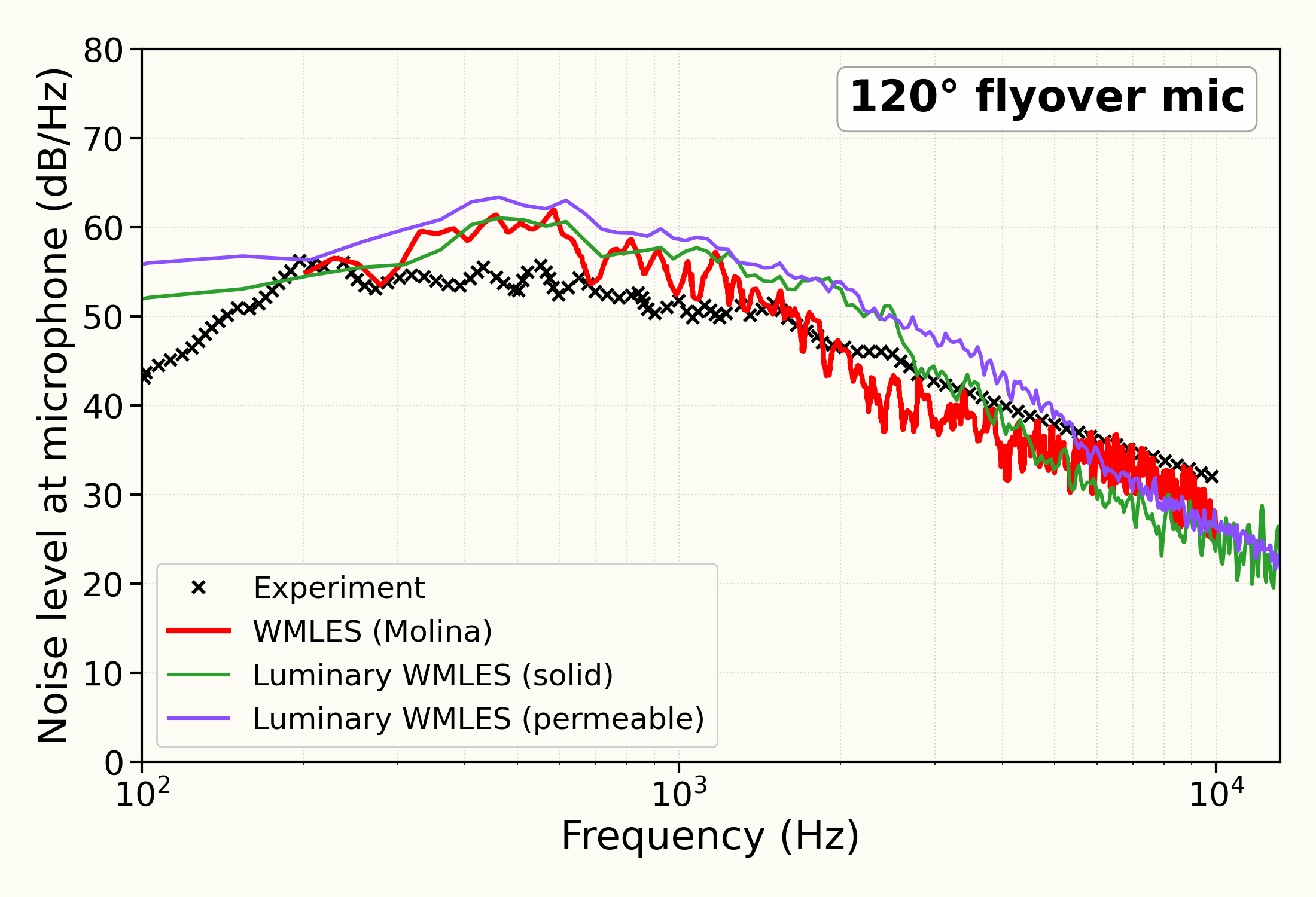
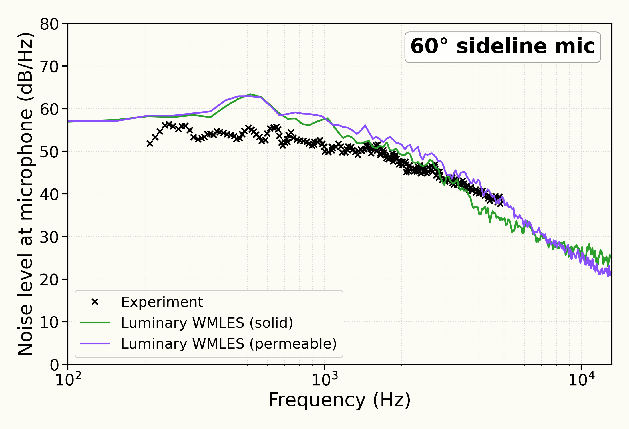
The far-field pressure spectra at the $60^{\circ}$ , $90^{\circ}$ and $120^{\circ}$ flyover and sideline observers, from the gear wall and from the permeable surface; the wall-pressure spectra at the kulite taps K9, K19, K1, K15 and K17; the mean pressure coefficient around the wheel; and the mean and RMS streamwise and vertical velocity along a line across the wake, each compared with the measurements of Manoha et al. (2008, 2009). The $120^{\circ}$ flyover spectrum and the spectra at K9 and K19 are also compared with the wall-modelled large-eddy simulation of Molina (2021). The velocity spectra at three points in the wake are shown against a $- 5 / 3$ power law.

Sources

E. Manoha, J. Bulté and B. Caruelle, “LAGOON: An Experimental Database for the Validation of CFD/CAA Methods for Landing Gear Noise Prediction,” 14th AIAA/CEAS Aeroacoustics Conference, AIAA Paper 2008-2816 (2008)., https://doi.org/10.2514/6.2008-2816

E. Manoha, J. Bulté, V. Ciobaca and B. Caruelle, “LAGOON: Further Analysis of Aerodynamic Experiments and Early Aeroacoustic Results,” 15th AIAA/CEAS Aeroacoustics Conference, AIAA Paper 2009-3277 (2009)., https://doi.org/10.2514/6.2009-3277

E. S. Molina, “Scale-resolving Methods in SU2,” 2nd Annual SU2 Conference, online presentation (September 2021)., https://www.youtube.com/watch?v=Smosy7FUm5Q

Results

Mean pressure coefficient around the wheel

Mean velocity in the wake

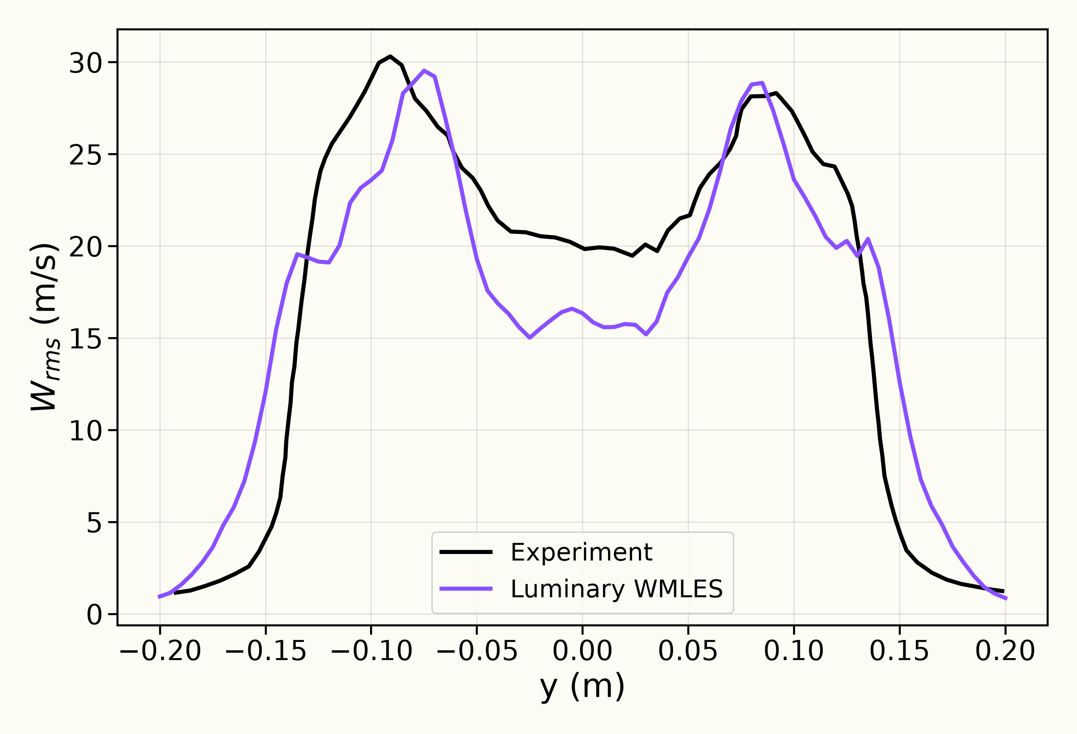
Mean streamwise velocity in the wake — Mean streamwise (left) and vertical (right) velocity along the transverse line at $x = 0.18$ m downstream of the wheels, against $y$ , with the measurements of Manoha et al. (2008, 2009). The vertical velocity is along $+ z$ , which points from the wheels toward the mount.

Mean vertical velocity in the wake — Mean streamwise (left) and vertical (right) velocity along the transverse line at $x = 0.18$ m downstream of the wheels, against $y$ , with the measurements of Manoha et al. (2008, 2009). The vertical velocity is along $+ z$ , which points from the wheels toward the mount.

RMS velocity in the wake

RMS streamwise velocity in the wake — RMS streamwise (left) and vertical (right) velocity along the transverse line at $x = 0.18$ m downstream of the wheels, against $y$ , with the measurements of Manoha et al. (2008, 2009). The vertical velocity is along $+ z$ , which points from the wheels toward the mount.

RMS vertical velocity in the wake — RMS streamwise (left) and vertical (right) velocity along the transverse line at $x = 0.18$ m downstream of the wheels, against $y$ , with the measurements of Manoha et al. (2008, 2009). The vertical velocity is along $+ z$ , which points from the wheels toward the mount.

Wake velocity spectra

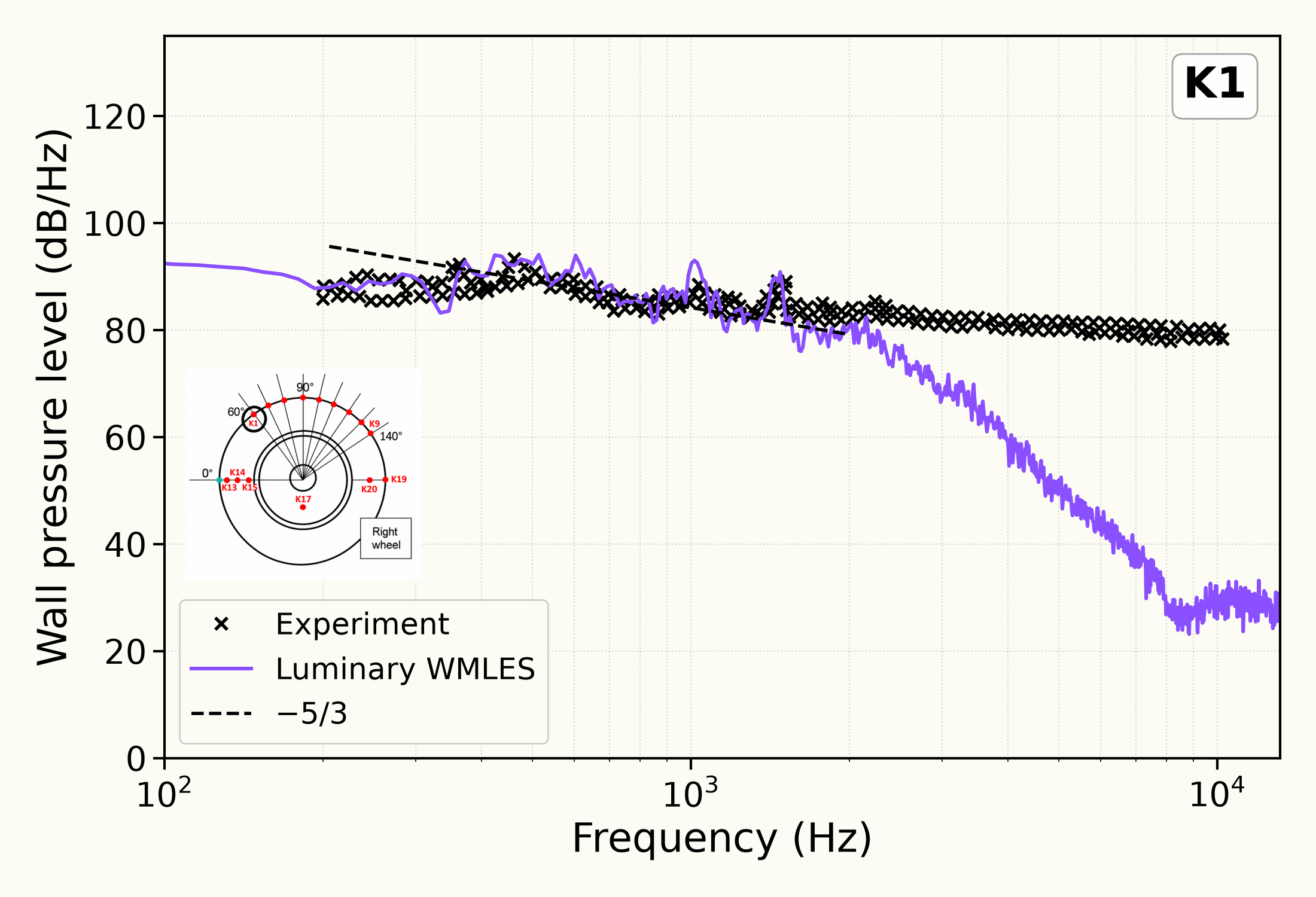
Wake streamwise velocity spectra — Power spectral density of the streamwise (left) and vertical (right) velocity fluctuation at the wake points $y = + 100$ , $0$ and $- 100$ mm, $x = 0.18$ m, $z = 0$ , with a $- 5 / 3$ power law fitted to the average of the three spectra between 200 Hz and 2 kHz.

Wake vertical velocity spectra — Power spectral density of the streamwise (left) and vertical (right) velocity fluctuation at the wake points $y = + 100$ , $0$ and $- 100$ mm, $x = 0.18$ m, $z = 0$ , with a $- 5 / 3$ power law fitted to the average of the three spectra between 200 Hz and 2 kHz.

Wall-pressure spectra at K1, K9 and K19

Wall-pressure spectrum at K1 — Power spectral density of the wall pressure at the kulite taps K1, K9 and K19, in dB re $(20 μ P a)^{2}$ /Hz, with the measurements of Manoha et al. (2008, 2009) and a $- 5 / 3$ power law fitted to the computed spectrum between 200 Hz and 1 kHz. K9 and K19 also show the wall-modelled large-eddy simulation (WMLES) of Molina (2021). Experiment (C19) and Experiment (F2) are the measurements in ONERA's CEPRA19 anechoic wind tunnel and in its F2 wind tunnel.

Wall-pressure spectrum at K9 — Power spectral density of the wall pressure at the kulite taps K1, K9 and K19, in dB re $(20 μ P a)^{2}$ /Hz, with the measurements of Manoha et al. (2008, 2009) and a $- 5 / 3$ power law fitted to the computed spectrum between 200 Hz and 1 kHz. K9 and K19 also show the wall-modelled large-eddy simulation (WMLES) of Molina (2021). Experiment (C19) and Experiment (F2) are the measurements in ONERA's CEPRA19 anechoic wind tunnel and in its F2 wind tunnel.

Wall-pressure spectra at K15 and K17

Wall-pressure spectrum at K15 — Power spectral density of the wall pressure at the kulite taps K15 and K17, in dB re $(20 μ P a)^{2}$ /Hz, with the measurements of Manoha et al. (2008, 2009) and a $- 5 / 3$ power law fitted to the computed spectrum between 200 Hz and 1 kHz.

Wall-pressure spectrum at K17 — Power spectral density of the wall pressure at the kulite taps K15 and K17, in dB re $(20 μ P a)^{2}$ /Hz, with the measurements of Manoha et al. (2008, 2009) and a $- 5 / 3$ power law fitted to the computed spectrum between 200 Hz and 1 kHz.

Far-field spectra at the flyover observers

Far-field spectrum at the $ 60^\circ $ flyover observer — Power spectral density of the acoustic pressure at the $60^{\circ}$ , $90^{\circ}$ and $120^{\circ}$ flyover observers, 6 m from the origin, from the FW-H analogy on the gear wall and on the permeable surface, in dB re $(20 μ P a)^{2}$ /Hz, with the measurements of Manoha et al. (2008, 2009). The $120^{\circ}$ observer also shows the wall-modelled large-eddy simulation (WMLES) of Molina (2021).

Far-field spectrum at the $ 90^\circ $ flyover observer — Power spectral density of the acoustic pressure at the $60^{\circ}$ , $90^{\circ}$ and $120^{\circ}$ flyover observers, 6 m from the origin, from the FW-H analogy on the gear wall and on the permeable surface, in dB re $(20 μ P a)^{2}$ /Hz, with the measurements of Manoha et al. (2008, 2009). The $120^{\circ}$ observer also shows the wall-modelled large-eddy simulation (WMLES) of Molina (2021).

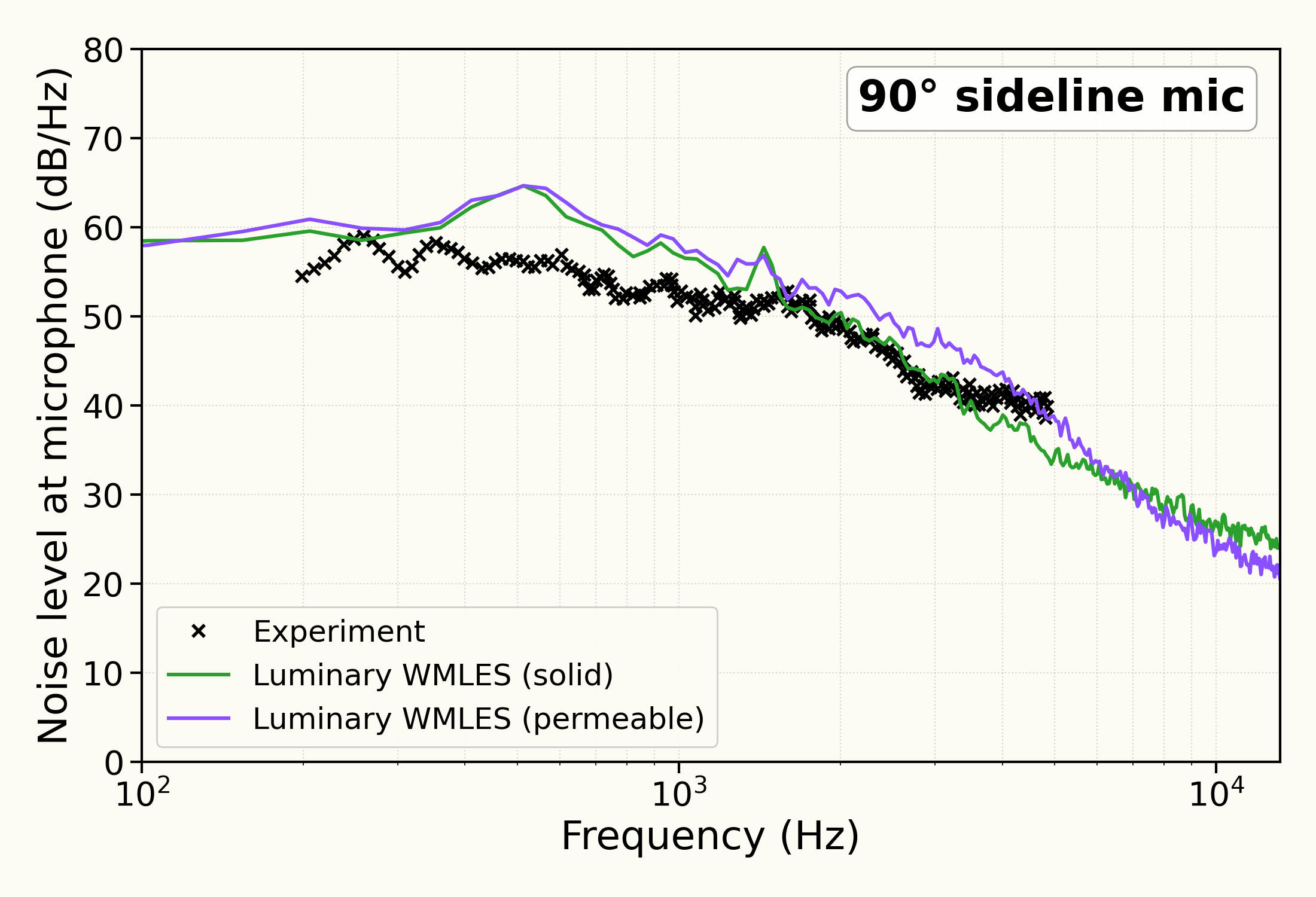
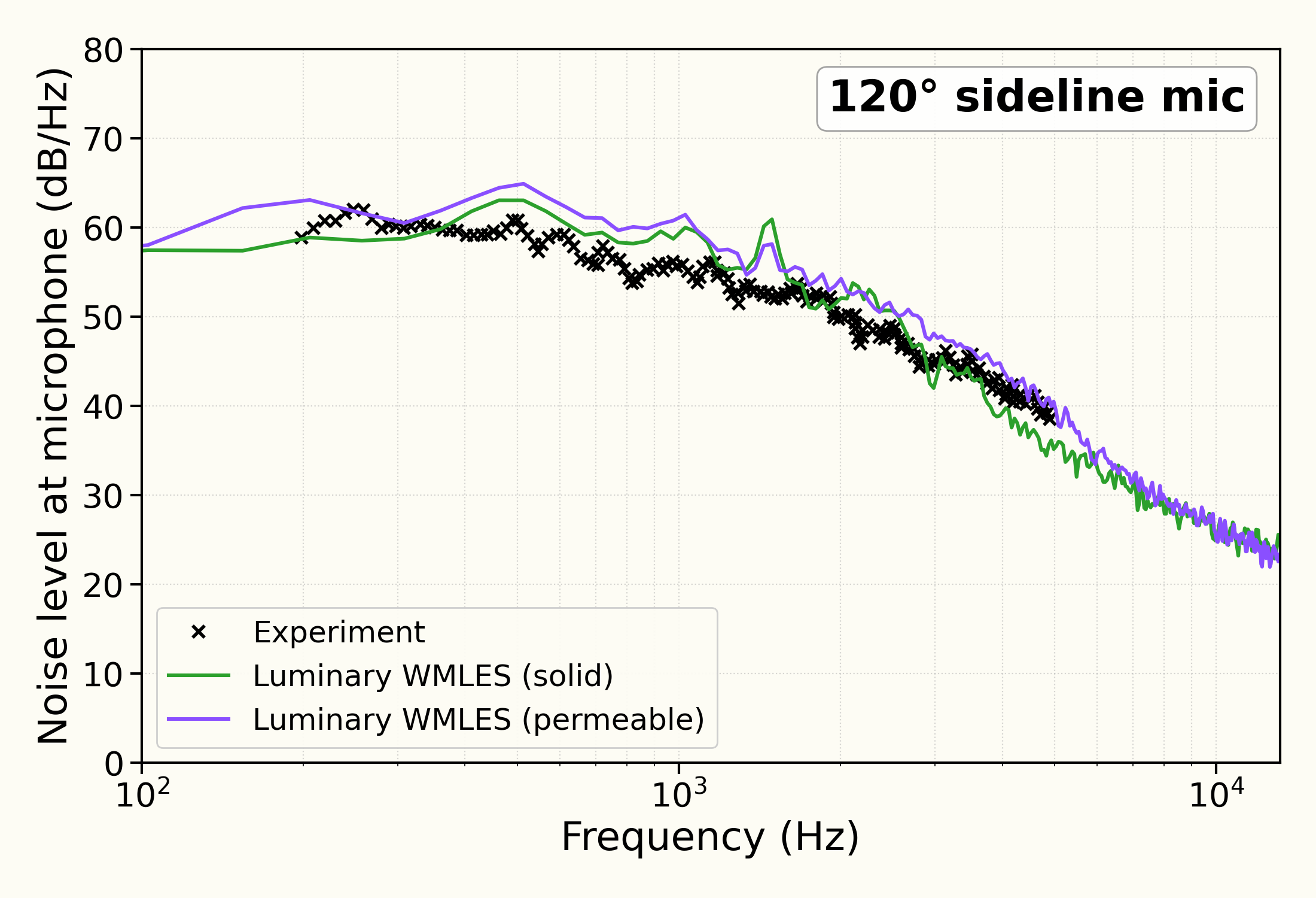
Far-field spectra at the sideline observers

Far-field spectrum at the $ 60^\circ $ sideline observer — Power spectral density of the acoustic pressure at the $60^{\circ}$ , $90^{\circ}$ and $120^{\circ}$ sideline observers, 6 m from the origin, from the FW-H analogy on the gear wall and on the permeable surface, in dB re $(20 μ P a)^{2}$ /Hz, with the measurements of Manoha et al. (2008, 2009).

Far-field spectrum at the $ 90^\circ $ sideline observer — Power spectral density of the acoustic pressure at the $60^{\circ}$ , $90^{\circ}$ and $120^{\circ}$ sideline observers, 6 m from the origin, from the FW-H analogy on the gear wall and on the permeable surface, in dB re $(20 μ P a)^{2}$ /Hz, with the measurements of Manoha et al. (2008, 2009).

Discussion

A landing gear has no single dominant tone. Its noise is a broad hiss from the turbulent wakes of the wheels, the axle and the leg, so the comparisons here are spectra: how loud the sound is at each frequency. The spectra are in decibels per hertz.

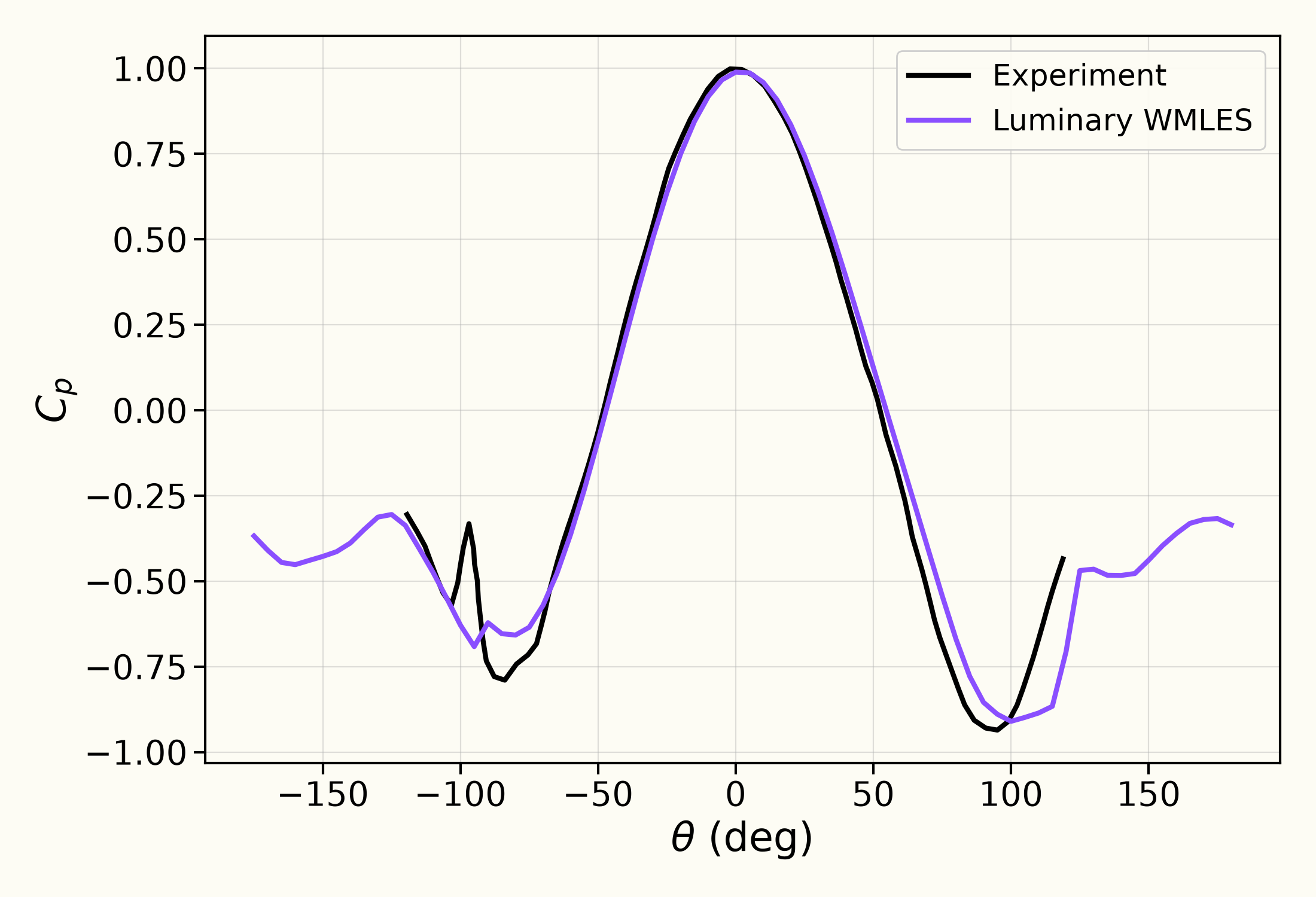
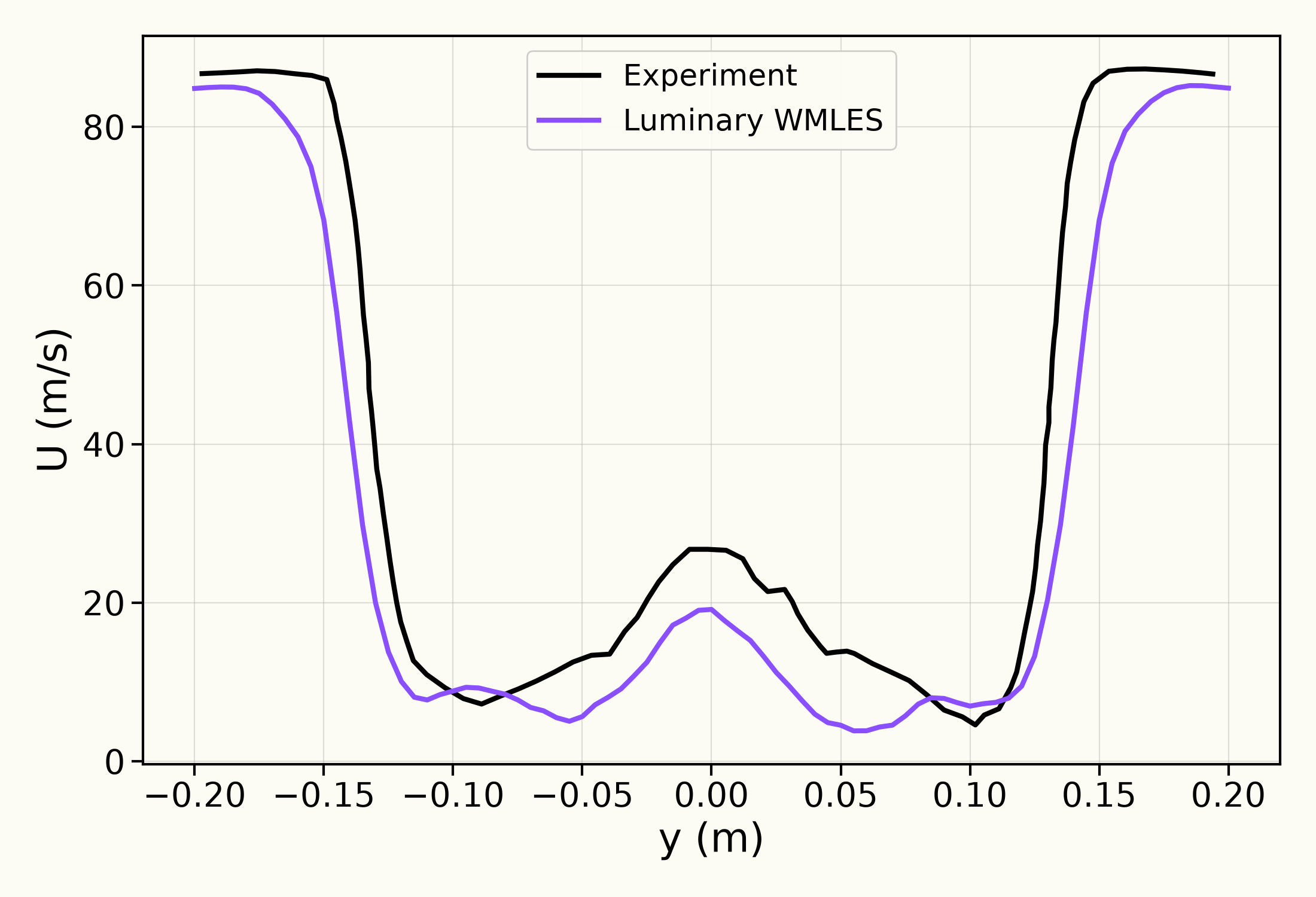
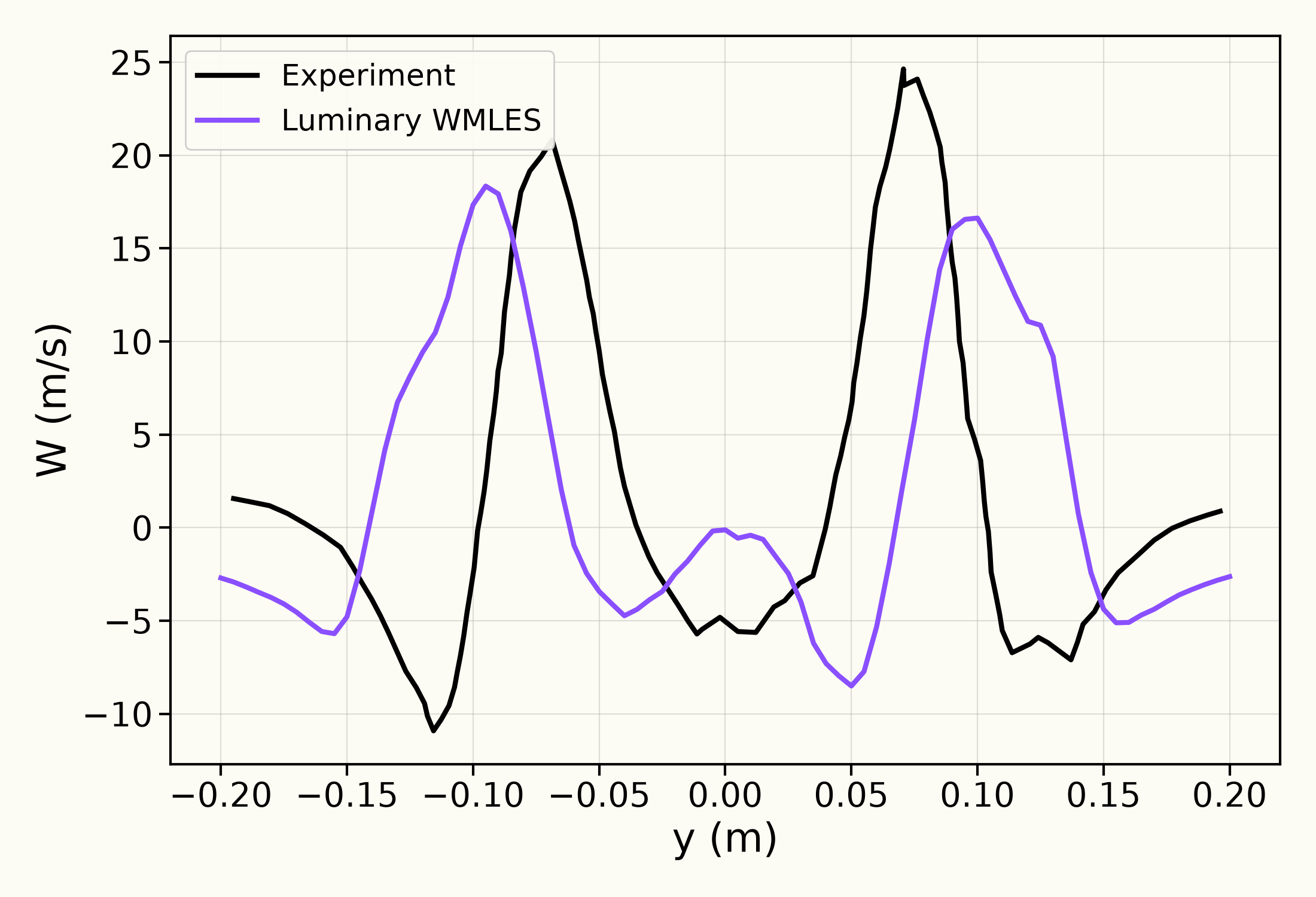
The flow around the gear comes first. The mean pressure follows the measurement over the front of the wheel. Behind the wheels the computed wake has the measured shape: a velocity deficit behind each wheel with faster flow between them, and the two upward peaks of the vertical velocity, with the computed wake slightly wider than the measured one.

The wall-pressure spectra at the kulite taps come straight from the flow solution. At each tap they follow the measurement from about $200$ Hz up to between $1.5$ and $4$ kHz depending on the tap, including the tones near $1$ kHz and $1.45$ kHz at K15. At K9 and K19 they are also close to the wall-modelled large-eddy simulation of Molina (2021).

At the far-field observers $6$ m away, both flyover and sideline, the Ffowcs Williams-Hawkings (FW-H) prediction from the gear wall follows the level and shape of the measured spectrum between about $200$ Hz and $2$ kHz, a few decibels above it around $500$ Hz. At the $120^{\circ}$ flyover observer it lies close to the simulation of Molina (2021), which shows the same rise around $500$ Hz. The permeable surface, which also takes in sound made in the wake around the gear, is a few decibels louder than the gear wall over most of this band.

Above a few kilohertz the computed spectra, like those of Molina (2021), fall below the measurement. The smallest eddies and the shortest sound waves a simulation can represent are a few grid cells across, so the mesh sets the highest frequency it resolves.

Solver configuration

features exercised: Validation 3D DES/LES Ideal gas Unsteady Energy equation FW-H (solid / permeable surface)